Relation extraction refers to the process of predicting and labeling semantic relationships between named entities. In this blog post, we’ll go over the process of building a custom relation extraction component using spaCy and Thinc. We’ll also add a Hugging Face transformer to improve performance at the end of the post. You’ll see how you can utilize Thinc’s flexible and customizable system to build an NLP pipeline for biomedical relation extraction.
In spaCy v3, we introduced a new, flexible training configuration system that gives you much more control over the various components in your NLP pipeline. You can integrate models written in any framework and build on pre-trained transformers that may significantly improve your accuracy. It’s also much easier to implement your own custom trainable component to solve any NLP task you’d like. If you’re interested in learning more about the changes implemented in spaCy v3, I recommend watching the introduction video, where Matt and Ines walk you through all the new features and concepts in detail.
This post offers a more practical viewpoint and shows how to apply the new spaCy v3 features as we work our way through implementing a new custom component from scratch. We will build a machine learning model in Thinc, implement a new spaCy component, train it with the new configuration system and demonstrate how to use a pre-trained transformer model from the Hugging Face Transformers library to boost your performance.
The specific challenge we are setting ourselves here is implementing a custom component to predict relationships between named entities, also called relation extraction. In the most basic form, we take two entities previously predicted by a named entity recognizer and try to determine whether there is a semantic relationship between them and, if so, label it.


Consider, for instance, a sentence with a Person entity and a Location entity: is the person living in that location, are they just visiting or are the two mentions unrelated? If you’re working with legal texts, you might want to connect the judge’s name to the correct case name. Or perhaps you’re parsing news articles in search of mergers and acquisitions and trying to understand the connections between various companies and individuals. There is no limit to the number of use-cases and domains relevant for relation extraction.
In this post, we’ll focus on predicting biomedical relations between genes and proteins. Biomedical NLP is a research area that I (Sofie) am passionate about, and I’ve worked in this domain extensively during my PhD and postdoc, now many years ago. For demonstration purposes, we’ve simplified the challenge and the annotation format quite a bit.
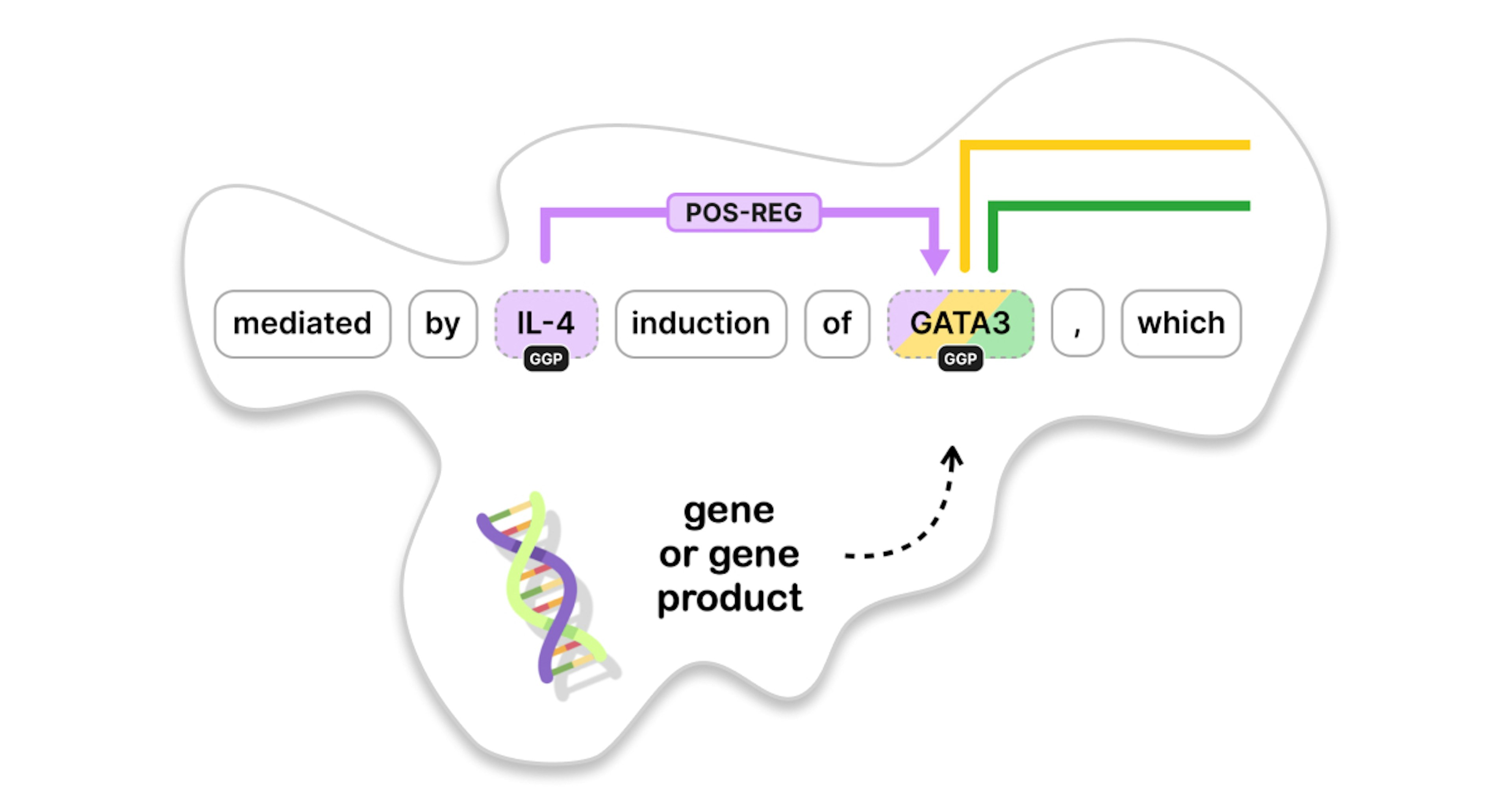
Genes are regions of your DNA that code for specific proteins. These proteins are responsible for many functions in your body: organizing cell growth, reacting to external impulses, fighting infections and so on. Take, for instance, this snippet describing the molecular mechanisms underlying allergy and asthma.

There are three entities marked as GGP, which stands for “gene or gene product”. We can annotate different relations between these entities, such as binding and regulatory associations. In the remainder of this post, we’ll assume that we have a named entity recognizer in place that detects the entities so that we can focus on the relations between them.
We start by creating a new spaCy pipeline component that predicts relationships between genes and proteins. This requires three main steps. First, we’ll build a machine learning model that takes a document as input and outputs the predicted relations. We’ll then use this model to power a pipeline component that integrates seamlessly within a normal spaCy pipeline. Once we’re done with the basic implementation, we’ll have a look at how to further enhance accuracy by using a pre-trained transformer from the Hugging Face Transformers library.
We will apply our relation extraction component to the use-case of biomolecular interactions, but you could adapt this approach to predict any type of relations between any type of entities. The performance of your relation extraction module will depend on the specific challenge and dataset, but keep in mind that predicting relations from text is a difficult task overall.
So let’s start with the first step of building the machine learning model. We’ll be using our own deep learning library, Thinc, which is lightweight and offers a functional programming API for composing neural networks. You could also use a different machine learning library, such as PyTorch or TensorFlow. The documentation has examples on wrapping such models for usage in spaCy.

This example document has just one sentence reading, “GATA3 inhibits FOXP3 expression”. This sentence has four tokens and two named entities referring to human genes. In the first step, we translate each token into a vector. To do this, we can use a standard Tok2Vec layer from spaCy or even a Transformer, as spaCy v3 fully interoperates with PyTorch and transformers, giving you access to thousands of pre-trained transformer models.
Here we show a simplified example where each token is encoded in a vector of length 5, but in reality, the width of these vectors should be much larger. Both entities in this text consist of only one token, which means that we can keep the token vector as such. If you had entities consisting of multiple tokens, we would need some sort of summarization method to obtain one final entity vector – for instance, by taking the average. We’ll come back to this later.
In the next step, we determine the candidate instances in our sentence. We are interested in direct, binary relations between two entities, which means that this sentence contains two relevant instances: one where “GATA3” is the object and “FOXP3” is the subject and one where it’s the other way around. For each instance, we simply concatenate the vectors of the two corresponding entities. At this point, you could also add additional features, but for now, we stick to these simple vectors where the first five numbers represent the subject, and the next set of five numbers represent the object.

We now concatenate all instance vectors into one larger tensor, which will be the input of our classification layer. Let’s assume we want to predict three relation types: binding, activation and inhibition. That means that the final output needs to contain a prediction for each instance and each relation type. The prediction scores will be between 0 and 1, and we consider everything above 0.5 as a True relation.
In our example where we have two instances and three unique labels, the final output is a 2x3 matrix, where the first row contains the predictions for the first instance. Ultimately, this allows us to determine a True or False value for each combination of an entity pair and a relation type.

Let’s translate this example into a schematic overview of the neural network. I’ve added type annotations to help clarify the type of data that flows through the different layers of the network. The input list of documents is first processed by the tok2vec layer, which produces a 2-dimensional matrix of floating point values for each document. We refer to this matrix as an object of type Floats2D. As the named entities in the document can consist of multiple tokens, we need a pooling layer that can summarize multiple vectors into one, for instance, by taking the mean.
In parallel, a get_instances function defines the pairs of entities in our documents that we want to label with relations. The type annotation here refers to Span objects, spaCy’s data structure that represents a slice of a document consisting of one or more tokens. A named entity in spaCy is stored internally as such a Span object, and each candidate relation is a tuple of two named entities.
The first layer of our network uses all this information to output the final tensor holding the instance data. Then, a classification layer transforms the instance data into the matrix holding the final predictions for each instance and each relation label. So how do we implement all of this in Thinc?
To create the relation extraction model, we define a function that takes the two main sublayers as arguments. First, the layer that creates the instance tensor. This layer is a Thinc Model that converts a list of documents to a 2-dimensional matrix. The second argument is the classification layer which converts the instance matrix into a predictions matrix. This modular approach will allow us to easily change parts of the model in future experiments.
The model architecture
Our relation extraction model is now defined by chaining the two sublayers together. This means that the output of the first layer will be fed as input to the next. We also define a custom attribute, get_instances, that refers to the corresponding attribute of the first layer. Later on, it will be useful to have a quick reference to this functionality.
Finally, we give this function a unique name and add it to spaCy’s architectures registry using the @spacy.registry decorator. This is a crucial new element in spaCy v3, which will allow us to reference this function in the configuration file when we train the model later on. The type annotations will support the validation of this configuration file.
The classification layer
But first, let’s dive deeper into the specifics of the two layers we need for our relation extraction model. Let’s start with the classification layer that takes an output dimension nO and an input dimension nI, and returns a Model that converts a 2D matrix into another 2D matrix. This layer does not necessarily have to be very complex. In fact, for now, we just define it as a Linear layer followed by a logistic output activation. This ensures that our predictions are within the [0,1] interval. Again, we register this layer as an architecture with a descriptive and unique name (rel_classification_layer.v1).
Until now, we’ve been able to just chain existing layers together, but things will become a bit more complex going forward. Let’s have a look at how to implement the first layer of our model, which creates the instance data from the raw text. As we mentioned earlier, you could also implement any of these layers in PyTorch or TensorFlow, but we wanted to take the opportunity of this tutorial to give you an example of how it could be done in Thinc.
Thinc is a bit different from other machine learning libraries and offers a functional take on deep learning. In Thinc, you define a layer in a neural network by implementing both its forward function, as well as its backpropagation. This powerful approach provides a lot of flexibility and transparency. The documentation has many technical details and background information. In this post, we’ll show you how the code looks in practice.
The model's forward function
We start by implementing the forward function, which takes a reference to a Thinc Model with the correct input and output types, then the input list of documents, and a boolean specifying whether we’re training or not. This is the standard signature of a forward function in Thinc.
As we’ve seen on the schematic overview, this layer needs access to three helper functions: a tok2vec layer to produce token vectors, a pooling layer to summarize multiple token vectors into one entity vector, and a get_instances function that will define the candidate instances in a document.
We first retrieve all instances in the input documents and then apply the tok2vec layer. This call returns not only the relevant token vectors but also a callback to perform the backpropagation of this specific step. This ensures that our tok2vec layer can be trained and tuned according to our relation extraction challenge. In spaCy v3, you can share such a tok2vec layer, or even a transformer, between different components, basically supporting multi-task learning and allowing your pipeline to run more efficiently by calculating these token vectors only once.
Next, we’ll build an explicit representation of the entities that will be part of our candidate relations.

Let’s first have a look at a more complex example with a multi-token entity. In this example, “TGF-beta” consists of 3 tokens. Each token is embedded as a vector with our tok2vec layer. Then, as before, we have two candidate instances in this sentence. The first instance has “TGF-beta” as the first entity, so we take all three relevant token vectors and we add the token vector of the second entity. The second instance represents the same relation but with the subject and object reversed, so we add the same rows but in a different order. In addition to building this matrix, we also keep track of the lengths of each entity: the first entity has length 3, while the second has length 1, and so on. This type of data structure, where we concatenate sequences that vary in the size of their first dimension, is actually quite common in NLP. Thinc has a special data structure called Ragged to easily deal with such variable-length sequence data while still keeping the data contiguous in memory.
Once we have created the Ragged object, Thinc provides several built-in operators to process this type of data. For instance, there is a standard pooling layer that will take the Ragged object, calculate the average of each entity, and return the result as a 2-dimensional matrix. In this new matrix, each entity is represented by just one row or one vector. We can horizontally stack the two entities for each instance, thus reshaping the matrix into the final instance tensor. In this tensor, each row now represents one relation instance.
The model's forward function (continued)
Let’s return to our code and implement this procedure. We’ll keep track of two lists: one storing the entity data and one storing the corresponding entity lengths. We loop through each document and obtain the corresponding candidate instances and token vectors. We then record all token indices that are a part of any of the entities in a specific relation instance. The length of each entity is stored as the number of tokens it contains.
We create the large matrix ents of all relevant vectors by retrieving the corresponding token vectors from the token indices. This is the array that we’ll use to create the Ragged object. The second argument we need for the Ragged constructor is the lengths array, and we make sure that this is of the proper type by casting it to a 1-dimensional array of integers. Now we can create the Ragged object with the array data and the list of lengths.
Having gone through this transformation, we now apply our pooling layer to the Ragged object and obtain a 2-dimensional array pooled with the entity vectors. Again, this call produces not only the resulting array but also an appropriate backpropagation callback bp_pooled that will allow us to revert the operation when we need to backpropagate the gradients to update the network.
In the final step, we reshape the matrix to obtain the tensor holding one candidate relation instance per row. The resulting relations array will now be returned by our forward function. And just like the other layers in Thinc, we’ll also return an appropriate backpropagation callback.
The backpropagation callback
The backpropagation function takes a gradient of outputs and computes the corresponding gradient of inputs. This is a crucial part of training your neural network and allowing your gradients to flow from the output layer all the way back to the input layer, meanwhile tuning your whole network. Thinc gives you full control over this backpropagation functionality.
First, we apply the pooling backpropagation callback bp_pooled. Next, we track the feedback for all entities and the relations they were a part of and propagate a summary of that feedback back to the token-level in d_tokvecs. Once we have this result, we apply bp_tokvecs, the backpropagation callback from the tok2vec layer, to those gradients. This will tell the tok2vec layer exactly where adjustments need to be made. Now that we have the forward function and its backpropagation callback, there are a few more minor details to take care of.
The initialization callback
Typically, a Thinc model defines an initialization callback that ensures that all internal weights and components are properly initialized before training begins. This method optionally takes a sample of input and output data (X and Y respectively) that is used to infer missing shapes and validate the network. For this particular model, we only need to ensure that the tok2vec layer is properly initialized.
Create tensors
Now we can put it all together and define the layer that generates the instance tensor from the raw text. Again, we adapt a modular approach by defining all required functions and sublayers as arguments: the tok2vec layer, the pooling layer and a get_instances function that defines our candidate instances. We call the Model constructor, give the model a name, refer to its forward function and its initialization function, and define the appropriate layers, references and attributes that we’ll need throughout the code base. Then we register this sublayer as an architecture in spaCy’s registry.
The instance generator
One detail that we haven’t discussed yet is the implementation of the get_instances function. This one really depends on your specific use case. It could be a function that pairs up any two entities in a document as long as they are within a certain maximum distance of each other. You could also define the set of candidate relations as any two entities that co-occur in the same sentence. If you make this function stricter, the model will have fewer instances to classify and will run more efficiently and probably with a higher precision rate, but at the cost of recall.
For the purpose of this tutorial, let’s create a simple function that takes a max_length argument, and that is added to spaCy’s misc registry, where you can register custom functions.
As you’ve seen throughout the code snippets, we have added all important functions to the spaCy registry. Now we’ll see how these are used in a configuration file. The configuration system is new in spaCy v3, and it’s a very powerful way to train and customize your NLP pipeline. The CLI command init config will help you hit the ground running. You just need to specify the language and components you’d like to train and optionally provide some more information about your goals and you’ll get a config file with reasonable defaults to start from.
Here, we’ll gradually build up a new configuration file for our relation extraction component and explain the different concepts to help you better understand how all of this works in practice.
config.cfg (excerpt)
Typically, there is an [nlp] section that defines the language and the components of your pipeline. In our case, the pipeline consists of just two parts: a tok2vec component and our relation_extractor component. We are not including a named entity recognizer at this point, and we’ll just use the gold-standard entities from the data. But in a realistic scenario, you’ll need to add one.
The configuration file further has a [components] section that allows you to define each component in more detail. Hierarchical sections are referenced with a dot notation.
config.cfg (excerpt)
For each component, a factory function is called, and its arguments should be specified in the same block. For instance, the built-in factory function for our tok2vec component will receive a model argument. In our configuration, this model refers to a registered architecture called spacy.HashEmbedCNN.v1. Note how the @ notation is used to access methods from a specific registry and with a specific name. The HashEmbedCNN architecture is a standard, built-in model, and it requires arguments such as width and depth. These function arguments are defined in the same block, as you see here.
One deliberate design choice that we’ve made in spaCy v3 is to avoid hidden default values in the code base. Ideally, all parameters of a model are defined in the configuration file, which greatly enhances transparency and reproducibility of your NLP experiments.
When this configuration file is passed on to the training command, all objects in it will be resolved in a bottom-up fashion. This means that it will first build the model architecture, validate its arguments and then pass the resulting object forward to the component factory, which will, in turn, create the actual component. This allows the configuration file to describe complex, nested trees of objects.
config.cfg (excerpt)
Our second component, the relation_extractor, refers to a similarly named factory that is not built-in, so we’ll implement it in a little bit. But it will receive a model defined by the architecture rel_model.v1, which is the machine learning model that we just implemented.
If you recall, this architecture chains together two sublayers: the first being the layer which creates the instance tensor, and which needs access to a tok2vec layer, a pooling layer, and a get_instances function, and a second layer which is the classification layer.
There is one additional pattern to highlight and clarify here. The tok2vec sublayer of the create_instance_tensor model refers to an architecture called Tok2VecListener. What this means in practice is that this sublayer will use the results from an upstream Tok2Vec component. This approach allows you to have only one Tok2Vec component in the pipeline but have multiple components built on top of it and tune it through backpropagation. You can apply the same pattern with a Transformer and a TransformerListener. If you have multiple components that could benefit from having a shared embedding layer, this new feature in spaCy v3 could improve both the accuracy as well as the speed of your pipeline.
Another convenient feature of this config system is that you can easily swap out parts of the configuration with different implementations by referring to a different layer or function with a different name in the registry. This gives developers a lot of flexibility to implement custom models and functionality.
But let’s circle back to the part where we refer to the relation_extractor component and its corresponding factory. In the next part of this blog post, we’ll show you how to implement a new trainable component from scratch and how to define this factory function. We will use the custom model we implemented in the first part to power the machine learning capabilities of our new component.
To implement a custom trainable component, you typically create a subclass of TrainablePipe. This component will hold a machine learning model that is defined in the configuration file. This schematic overview depicts the main functions we need to implement to obtain a fully functional component. Let’s have a quick look at them before we dive into the details of the code.

The constructor of the component is typically invoked through a factory function and receives a Thinc Model. You can also implement your machine learning model in Tensorflow or PyTorch and wrap it with one of the available wrappers in Thinc.
The initialize method of a component should be called right after creation and before training begins. This method is usually triggered by invoking nlp.initialize. It ensures that the component and its internal model are properly set up, for instance, by defining the set of labels or by inferring the input and output dimensions of the neural network from sample data. Note that this initialization step only happens before the component has been trained. Once the model is trained and loaded back in from disk, this function will not be relevant anymore. The configuration file has a corresponding section called initialize that may hold relevant information for this step.
Once the component is created and initialized, we can start training the internal machine learning model. This is done by the update method, which receives a batch of training data encoded in Example objects. Example is a new type of object in spaCy v3 and replaces the old GoldParse. We’re actually quite happy about this refactor because the new data structure is much easier and transparent to work with. An Example holds both a document with predictions, as well as a document called reference that has the gold-standard annotations. The update method will first create predictions with the current model and then compare them to the gold-standard data to calculate the loss and tune the model further through backpropagation.
Once the model is trained, the predict method will produce predictions. This method typically delegates to the internal machine learning model and returns the predicted scores. If you want to store the results in the document, the function set_annotations should be called right after. In fact, the __call__ method does exactly that: it produces the predictions with predict , then calls set_annotations to store them.
To speed up processing of a larger set of documents, TrainablePipe has a standard implementation of a pipe method that processes the documents in batches. This method also delegates to predict and set_annotations.

For our relation extraction component, we will store the final predictions for a document in the custom attribute doc._.rel. As keys, we represent an instance pair by the start offsets of the two entities, which is a unique key within one document. Each key then refers to another dictionary that maps each relation label to a score between 0 and 1.
When we feed gold-standard training data into our relation component, these annotations will be stored in the Example object’s reference document in a similar way. In comparison to spaCy v2, this gives you a lot of flexibility on how to define gold-standard annotations. You only need an internal convention on how to store the data on the document, and that’s exactly what the custom attributes can be used for.
Now let’s dive into the code for more detail. Here is the skeleton of the pipeline component, containing all the main functions that we need to implement.
Skeleton of the relation extraction component
The constructor requires a reference to the vocab instance of the pipeline, as well as the name of the component we’re creating. But the most important bit here is that it receives a machine learning model as an argument and stores it internally as self.model. For our use case, this will be the Thinc Model that we implemented in the first part of this tutorial.
def __init__(self, vocab, model, name: str = "rel"): self.vocab = vocab self.model = model self.name = name self.cfg = {"labels": []}Much like other pipeline components such as Tagger or TextCategorizer, we need an internal list of labels. For now, this is an empty list. We implement a property to access these labels easily, and we also provide a convenience method to add a label.
@propertydef labels(self) -> Tuple[str]:    return tuple(self.cfg["labels"])
def add_label(self, label: str):    self.cfg["labels"] = list(self.labels) + [label]
We can now implement the component factory that will be referred to from the configuration file. Component factories can be registered with the @Language.factory decorator, and they always take the nlp object and the component’s name as arguments. As we’ve seen, the constructor of our relation extractor component also needs a machine learning model. The factory then calls the constructor and returns the new object.
@Language.factory("relation_extractor")def make_relation_extractor(nlp, name, model): return RelationExtractor(nlp.vocab, model, name)After creating the pipeline component, we need to initialize it. The relevant code is shown here.
First, we make sure that the labels are properly defined. There are two ways to do this. The first way is to provide the list of labels explicitly in the variable labels by defining them in the initialize section of the config. The other option is more of an implicit one: it derives all labels from the gold-standard data that is provided as argument to this method. The relevant labels can be retrieved from the custom attribute doc._.rel.
After defining the labels, we call the internal model’s initialization method with the input documents and the corresponding output predictions. This allows Thinc to perform shape inference and validation and ensures that all layers are ready to start training.
def initialize(self, get_examples, *, nlp=None, labels=None): examples = get_examples() if labels is not None: for label in labels: self.add_label(label) else: for eg in examples: doc = eg.reference relations = doc._.rel for indices, label_dict in relations.items(): for label in label_dict.keys(): self.add_label(label) docs = [eg.reference for eg in examples] labels = self._examples_to_truth(examples) self.model.initialize(X=docs, Y=labels)Training a model is done by invoking the method update. We focus on the main implementation parts here and refer to the projects repository, which has the full code.
def update(self, examples, *, drop=0.0, set_annotations=False, sgd=None, losses=None): docs = [eg.predicted for eg in examples] predictions, backprop = self.model.begin_update(docs) loss, gradient = self.get_loss(examples, predictions) backprop(gradient) losses[self.name] += loss return lossesWe first fetch all the documents containing predictions from the list of example objects. We then run these documents through the internal model by calling model.begin_update. This method returns the predictions, as well as a backpropagation callback. The predictions are then compared to the actual gold-standard annotations. The component’s get_loss method calculates the loss for this batch of examples, as well as the gradient of the loss. This gradient is provided as argument to the backpropagation function that will update the internal weights of the model layers. At the end, we update the losses dictionary and return it.
The get_loss method that we just used can be implemented any way you like – in this case, we’ve opted for a simple mean square error, as shown here.
def get_loss(self, examples, scores): truths = self._examples_to_truth(examples) gradient = scores - truths mean_square_error = (gradient ** 2).sum(axis=1).mean() return float(mean_square_error), gradientOnce the model is trained, the component can be used to make novel predictions. The predict method delegates its work to the internal model that takes a batch of Doc objects and returns an array with the predicted scores.
def predict(self, docs): return self.model.predict(docs)The final method that needs to be implemented is set_annotations. This method takes the array with predicted scores, interprets it and modifies the Doc objects in place with the correct annotations. This is what happens behind the scenes when you call nlp on a string of text: each pipeline component is called on the Doc passing through the pipeline, and each component sets its predictions accordingly.
def set_annotations(self, docs, scores): c = 0 get_instances = self.model.attrs["get_instances"] for doc in docs: for (e1, e2) in get_instances(doc): offset = (e1.start, e2.start) if offset not in doc._.rel: doc._.rel[offset] = {} for j, label in enumerate(self.labels): doc._.rel[offset][label] = scores[c, j] c += 1To make sure that we interpret the scores correctly, we need to refer to the model’s get_instances function that defines the list of instances in each document. As you may recall, an instance is represented by the start offsets of its two entities. For each relation label, we then record the score of that specific label for that specific relation in our custom attribute.
With this, we have implemented the most important parts of our relation extractor component, and we will soon be able to put it to use. As a quick recap, recall that this implementation required two main parts. First, we implemented a machine learning model from scratch, using our library Thinc. We managed the forward and backward passes of our neural network to ensure that all layers are tuned for our specific challenge. Then we implemented a trainable pipeline component that uses this machine learning model to make predictions and store them on the document. We can use this component as part of any NLP pipeline in spaCy. Ideally, it is combined with a trainable named entity recognizer that is specific to your challenge as well.
In the remainder of this post, we’ll look at some results of running this pipeline component on a custom dataset that we’ve annotated with Prodigy. We will use an example spaCy project that runs the full workflow.
Additionally, we will show you how to swap out the standard tok2vec component and use a pre-trained transformer from the Hugging Face Transformers library instead – and we’ll see how that impacts performance levels. If you’ve followed the recent hype in NLP on transformer models, you can probably make an informed guess on how they’ll impact accuracy.
Throughout this post, we’ve focused on the most important bits of code and skipped a few implementation details. However, we’ve released the full code base so you can inspect it further in detail. For instance, the full code also includes a scoring function for calculating F-scores for our relation extraction component, a few helper functions, and some error handling to make the code more robust. The code for this component is released as a spaCy project. spaCy projects is another cool feature of spaCy v3. It is a repository that lets you manage and share end-to-end NLP workflows for different use cases and domains. You can simply clone a pre-defined project template, run it, inspect it, play with it and adapt it to fit your needs.
The full project contains gold-standard data that we created with our annotation tool, Prodigy. Prodigy is a scriptable annotation tool that offers several built-in annotation recipes, such as the rel.manual recipe that was released with Prodigy v1.10. This recipe allows you to annotate entities and relations at the same time.

In our case, GGP entities are predefined in the dataset and left as-is, and we only focus on getting the relations between these entities correct. We have annotated a small set of articles from the BioNLP Shared Task 2011, where the texts are taken from PubMed and PubMed Central. We export these annotations as a JSONL file and include it in the project as a data asset.
A spaCy project always has a project.yml file that defines the typical workflow and scripts that should be run in sequence. I won’t go into the details here, but let’s run through the workflow with spaCy projects.
First, the JSONL file from Prodigy, containing the gold-standard data, is parsed into the new binary format with extension .spacy. These binary files are actually pretty easy to generate: you parse the annotations and create Doc objects that store the information in the custom attribute, as we’ve seen before. These documents are stored to disk using the DocBin class, which provides efficient serialization of a collection of Doc objects.
After parsing the data, we use the training set to train the model and the dev set to evaluate the F-score throughout the training loop. The model with the best F-score is then selected and applied to a held-out test set for a final evaluation.
If we assume a cutoff of 0.5 for predictions to be True, our best model obtains about 42% F-score. Note that typically, relation extraction challenges suffer from highly imbalanced datasets, as most candidate instances are usually negatives, so it is challenging to obtain high F-scores. It would certainly be worthwhile to try and extend this basic model to incorporate more features and enhance the prediction power. And it wouldn’t hurt to annotate some more data, either.
One final spaCy v3 feature that we would like to show you is how to use a transformer instead of a standard tok2vec layer. You’ll need to install our plugin spacy-transformers, which provides full integration with all the pre-trained models in the Hugging Face Transformers library.
Let’s revisit the config file we’ve defined before. Instead of the tok2vec component, we’ll now have a transformer in the pipeline. This transformer is defined by its own factory, which requires some additional arguments – we’ll just use the default values here and refer to the documentation for details.
config.cfg (excerpt)
You’ll want to use the built-in architecture TransformerModel and give it the name of one of the pre-trained Hugging Face models you’d like to use and tune.
We also need to adjust the definition of our relation extraction model slightly. Specifically, the tok2vec sublayer will now refer to a TransformerListener that connects to the transformer component in the pipeline to obtain the token vectors. You can have multiple components, all listening to the same transformer model and all passing gradients back to it. This effectively enables multi-task learning. By default, all of the gradients will be equally weighted, but you can control this with the grad_factor setting.
config.cfg (excerpt)
As transformer models provide wordpiece vectors, we’ll need a pooling layer to obtain token vectors from the word pieces. We just apply the same reduce_mean layer that we also applied to summarize token vectors into entity vectors. This layer is a built-in component from Thinc, but you could pick any other one or implement your own strategy as well.
There are a few additional changes that we have to make when switching over from the tok2vec layer to the transformer. For instance, we change the batching strategy of the training loop, and we also adjust the learning rate to obtain reasonable results. These details can be inspected by comparing both the configuration files in the projects repo. If you’re wondering what sensible default parameters are in general, you can run the CLI command init config and obtain recommended settings for your use-case. This is usually a good place to start – but you’ll want to do some parameter tuning for your specific data and challenge.
We can store the configuration file with the transformer under a new name and run it in the spaCy project by invoking a different workflow. You will need a decent GPU to be able to train this model, but it’s worth it! The final F-score of our best model on the test set is around 72%, which is 30 percentage points higher than our initial result. This illustrates that on small datasets specifically, leveraging a pre-trained transformer model can significantly boost your performance.
We hope you’ve enjoyed reading this blog post in which we discussed the practical steps to implement your own trainable component in spaCy v3. We saw how to build a model with Thinc, how to use the new configuration system, how to implement a new pipeline component, and how to use a transformer to boost the performance of your pipeline.
If you are specifically interested in implementing a relation extraction component for your domain, you can clone the code from our projects repo and give it a spin. Please consider this approach as a very first baseline. You’ll probably want to extend it further with more features and better data. Let us know how it goes in the discussions forum!