- 14 minute read
- Blog
- Embeddings & Vectors

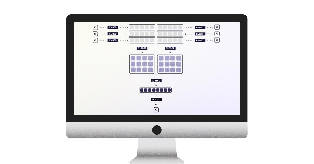
Over the last six months, a powerful new neural network playbook has come together for Natural Language Processing. The new approach can be summarised as a simple four-step formula: embed, encode, attend, predict. This post explains the components of this new approach, and shows how they’re put together in two recent systems.
Update (January 2018)
spaCy v2.0 now features deep learning models for named entity recognition, dependency parsing, text classification and similarity prediction based on the architectures described in this post. You can now also create training and evaluation data for these models with Prodigy, our new active learning-powered annotation tool. See this video for an example of training an NER system using Prodigy.
When people think about machine learning improvements they usually think about efficiency and accuracy, but the most important dimension is generality. If you want to write a program to flag abusive posts on your social media platform, you should be able to generalise the problem to “I need to take text and predict a class ID”. It shouldn’t matter whether you’re flagging abusive posts or tagging emails that propose meetings. If two problems take the same type of input and produce the same type of output, we should be able to reuse the same model code, and get a different behaviour by plugging in different data — like playing different games that use the same engine.
Let’s say you have a great technique for predicting a class ID from a dense vector of real values. You’re convinced you can solve any problem that has that particular input/output “shape”. Separately, you also have a great technique for predicting a single vector from a vector and a matrix. Now you have the solutions to three problems, not two. If you start with a matrix and a vector, and you need a class ID, you can obviously compose the two techniques. Most NLP problems can be reduced to machine learning problems that take one or more texts as input. If we can transform these texts to vectors, we can reuse general purpose deep learning solutions. Here’s how to do that.
A four-step strategy for deep learning with text
Embedded word representations, also known as “word vectors”, are now one of the most widely used natural language processing technologies. Word embeddings let you treat individual words as related units of meaning, rather than entirely distinct IDs. However, most NLP problems require understanding of longer spans of text, not just individual words. There’s now a simple and flexible solution that is achieving excellent performance on a wide range of problems. After embedding the text into a sequence of vectors, bidirectional RNNs are used to encode the vectors into a sentence matrix. The rows of this matrix can be understood as token vectors — they are sensitive to the sentential context of the token. The final piece of the puzzle is called an attention mechanism. This lets you reduce the sentence matrix down to a sentence vector, ready for prediction. Here’s how it all works.
Step 1: Embed
An embedding table maps long, sparse, binary vectors into shorter, dense,
continuous vectors. For example, imagine we receive our text as a sequence of
ASCII characters. There are 256 possible values, so we can represent each value
as a binary vector with 256 dimensions. The value for a will be a vector of
0s, with a 1 at column 97, while the value for b will be a vector of zeros
with a 1 at column 98. This is called the “one hot” encoding scheme. Different
values receive entirely different vectors.

Most neural network models begin by tokenising the text into words, and embedding the words into vectors. Other models extend the word vector representation with other information. For instance, it’s often useful to pass forward a sequence of part-of-speech tags, in addition to the word IDs. You can then learn tag embeddings, and concatenate the tag embedding to the word embedding. This lets you push some amount of position-sensitive information into the word representation. However, there’s a much more powerful way to make the word representations context-specific.
Step 2: Encode
Given a sequence of word vectors, the encode step computes a representation that I’ll call a sentence matrix, where each row represents the meaning of each token in the context of the rest of the sentence.

The technology used for this purpose is a bidirectional RNN. Both LSTM and GRU architectures have been shown to work well for this. The vector for each token is computed in two parts: one part by a forward pass, and another part by a backward pass. To get the full vector, we simply stick the two together. Here’s what’s being computed:
Bidirectional RNN
I think bidirectional RNNs will be one of those insights that come to feel obvious with time. However, the most direct application of an RNN is to read the text and predict something from it. What we’re doing here is instead computing an intermediate representation — specifically, per token features. Crucially, the representation we’re getting back represents the tokens in context. We can learn that the phrase “pick up” has a different meaning from the phrase “pick on”, even if we processed the two phrases into separate tokens. This has always been a huge weakness of NLP models. Now we have a solution.
Step 3: Attend
The attend step reduces the matrix representation produced by the encode step to a single vector, so that it can be passed on to a standard feed-forward network for prediction. The characteristic advantage of an attention mechanism over other reduction operations is that an attention mechanism takes as input an auxiliary context vector:

By reducing the matrix to a vector, you’re necessarily losing information. That’s why the context vector is crucial: it tells you which information to discard, so that the “summary” vector is tailored to the network consuming it. Recent research has shown that the attention mechanism is a flexible technique, and new variations of it can be used to create elegant and powerful solutions. For instance, Parikh et al. (2016) introduce an attention mechanism that takes two sentence matrices, and outputs a single vector:

Yang et al. (2016) introduce an attention mechanism that takes a single matrix and outputs a single vector. Instead of a context vector derived from some aspect of the input, the “summary” is computed with reference to a context vector learned as a parameter of the model. This makes the attention mechanism a pure reduction operation, which could be used in place of any sum or average pooling step.
Step 4: Predict
Once the text or pair of texts has been reduced into a single vector, we can learn the target representation — a class label, a real value, a vector, etc. We can also do structured prediction, by using the network as the controller of a state machine such as a transition-based parser.

Interestingly, most NLP models usually favour quite shallow feed-forward networks. This has meant that some of the most important recent technologies for computer vision, such as residual connections and batch normalisation have so far had relatively little impact in the NLP community.
Example 1: A Decomposable Attention Model for Natural Language Inference
Natural language inference is a problem of predicting a class label over a pair of sentences, where the class represents the logical relationship between them. The Stanford Natural Language Inference corpus uses three class labels:
- Entailment: If the first sentence is true, the second sentence must be true.
- Contradiction: If the first sentence is true, the second sentence must be false.
- Neutral: Neither entailment nor contradiction.
Bowman et al. (2015) give the following examples from the corpus:
| Text | Hypothesis | Label |
|---|---|---|
| A man inspects the uniform of a figure in some East Asian country. | The man is sleeping | contradiction |
| An older and younger man smiling. | Two men are smiling and laughing at the cats playing on the floor. | neutral |
| A black race car starts up in front of a crowd of people. | A man is driving down a lonely road. | contradiction |
| A soccer game with multiple males playing. | Some men are playing a sport. | entailment |
One of the motivations for the corpus is to provide a new, reasonably sized corpus for developing models that encode sentences into vectors. For example, Bowman et al. (2016) describe an interesting transition-based model that reads a sentence sequentially to construct a tree-structured internal representation.
Bowman et al. were able to achieve an accuracy of 83.2, a substantial improvement over previous work. Less than six months later, Parikh et al. (2016) presented a model that achieved 86.8% accuracy, with around 10% of the parameters of Bowman et al.’s model. Soon after, Chen et al. (2016) published a system that performed even better — 88.3%. When I first read Parikh et al.’s paper, I couldn’t understand how their model performed so well. The answer is in the way the model mixes the two sentence matrices, using their novel attention mechanism:

The crucial advantage is that the sentence-to-vector reduction operates over he sentences jointly, while Bowman et al. (2016) encode the sentences into vectors independently. Remember Vapnik’s princple:
When solving a problem of interest, do not solve a more general problem as an intermediate step.
Parikh et al. (2016) take the natural language inference task to be the problem of interest. They structure their problem to solve it directly, and therefore have a big advantage over models which encode the sentences separately. Bowman et al. are more interested in the general problem, and structure their model accordingly. Their model is therefore useful in situations where Parikh et al.’s is not. For instance, with Bowman et al.’s model, you cache the sentence vector, making it much more efficient to compute a similarity matrix.
Example 2: Hierarchical Attention Networks for Document Classification
Document classification was the first NLP application I ever worked on. The Australian equivalent of the SEC funded a project to crawl Australian websites and automatically detect financial scams. While the project was a little ahead of its time, document classification changed surprisingly little over most of the next ten years. That’s why I find the hierarchical attention networks model that Yang et al. (2016) recently published so exciting. It’s the first paper I’ve seen to offer a really compelling general improvement over older bag-of-words models. Here’s how it works.
The model receives as input a document, consisting of a sequence of sentences, where each sentence consists of a sequence of word IDs. Each word of each sentence is separately embedded, to produce two sequences of word vectors, one for each sentence. The sequences are then separately encoded into two sentence matrices. An attention mechanism then separately reduces the sentence matrices to sentence vectors, which are then encoded to produce a document matrix. A final attention step reduces the document matrix to a document vector, which is then passed through the final prediction network to assign the class label.

This model uses the attention mechanism as a pure reduction step: it learns to take a matrix as input, and summarise it into a vector. It does this by learning context vectors for the two attention transformations, which can be understood as representing words or sentences that the model would find ideally relevant. Alternatively, you can see the whole reduction step as a feature extraction procedure. Under this view, the context vector is just another opaque parameter.
| Author | Methods | Yelp ‘13 | Yelp ‘14 | Yelp ‘15 | IMDB |
|---|---|---|---|---|---|
| Yang et al. (2016) | HN-ATT | 68.2 | 70.5 | 71.0 | 49.4 |
| Yang et al. (2016) | HN-AVE | 67.0 | 69.3 | 69.9 | 47.8 |
| Tang et al. (2015) | Paragraph Vector | 57.7 | 59.2 | 60.5 | 34.1 |
| Tang et al. (2015) | SVM + Bigrams | 57.6 | 61.6 | 62.4 | 40.9 |
| Tang et al. (2015) | SVM + Unigrams | 58.9 | 60.0 | 61.1 | 39.9 |
| Tang et al. (2015) | CNN-word | 59.7 | 61.0 | 61.5 | 37.6 |
An interesting comparison can be drawn between the Yang et al. (2016) model and a convolutional neural network (CNN). Both models are able to automatically extract position-sensitive features. However, the CNN model is both less general and less efficient. With the bidirectional RNN, each sentence only needs to be read twice — once forwards, and once backwards. The LSTM encoding can also extract features of arbitrary length, because any aspect of the sentence context might be mixed into the token’s vector representation. The procedures for reducing the sentence matrix to a vector is also simple and efficient. To construct the document vector, the same procedure is simply applied again.
The main factor that drives the model’s accuracy is the bidirectional LSTM encoder, to create the position-sensitive features. The authors demonstrate this by swapping the attention mechanism out for average pooling. With average pooling, the model still outperforms the previous state-of-the-art on all benchmarks. However, the attention mechanism improves performance further on all evaluations. I find this especially interesting. The implications are quite general — there are after all plenty of situations where you want to reduce a matrix to a vector for further prediction, without reference to any particular external context.
Next Steps
I’ve implemented the entailment model for use with our NLP library, spaCy, and I’m working on an implementation of the text classification system. We’re also planning to ship a general-purpose bidirectional LSTM model for use with spaCy, to make it easy to use pre-trained token vectors on your problems.
Update (January 2018)
spaCy v2.0 now features deep learning models for named entity recognition, dependency parsing, text classification and similarity prediction based on the architectures described in this post. You can now also create training and evaluation data for these models with Prodigy, our new active learning-powered annotation tool. See this video for an example of training an NER system using Prodigy.
Bibliography
- Decomposable Attention Model for Natural Language Inference Parikh, Ankur P.; Tackström, Oscar; Das, Dipanjan; Uszkoreit, Jakob (2016)
- Enhancing and Combining Sequential and Tree LSTM for Natural Language Inference Chen, Qian; Zhu, Xiaodan; Ling, Zhenhua; Wei, Si (2016)
- Hierarchical Attention Networks for Document Classification Yang, Zichao; Yang, Diyi; Dyer, Chris; He, Xiaodong; Smola, Alex; Hovy, Eduard (2016)
- A Fast Unified Model for Parsing and Sentence Understanding Bowman, Samuel R.; Gauthier, Jon; Rastogi, Abhinav; Gupta, Raghav; Manning, Christopher D.; Potts, Christopher (2016)
- A large annotated corpus for learning natural language inference Bowman, Samuel R.; Angeli, Gabor; Potts, Christopher; Manning, Christopher D. (2015)
- Semi-supervised Convolutional Neural Networks for Text Categorization via Region Embedding Johnson, Rie; Zhang, Tong (2015)


