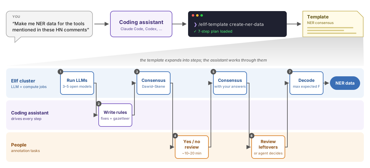
We present a workflow to cheaply acquire high-quality named entity recognition training or evaluation data using open-weight models. The workflow gets a coding agent such as Claude Code to drive a multi-step process, following a template to keep it on track.
Equipped with a Kubernetes-based execution environment and a toolkit for configuring efficient annotation UIs, the agent sends work to multiple small LLMs or NER models, integrates their annotations using a consensus algorithm, designs and adds rule-based post-processing or gazetteer matching, assigns efficient binary-decision annotation tasks to human annotators, and requests manual review of remaining uncertainties.
We evaluate this workflow by creating two small NER corpora, one
with an arbitrary task-specific category (identifying tools and technologies
in Hacker News posts), and the other tagging news text with four standard NER
categories (PERSON, ORG, PRODUCT, GPE). We ran 3–5 open-weight models over
the evaluation sets, prompted the coding assistant to develop rules and
terminology lists, and used the consensus algorithm to calculate a single
best output that tied GPT 5.6 Sol on one task and outperformed it on the other,
at 1/25th the runtime cost. We then performed 10–20 minutes of annotation
on the most uncertain examples, producing data with 50–60% fewer errors than
GPT 5.6 Sol’s output on both tasks.
What’s the point?
Span labeling tasks (NER, etc.) are surprisingly hard for LLMs. Recent large frontier models are now getting quite good results, but they’re too expensive for many production workloads, and most commercial providers (Anthropic, Google, others) prohibit using their models to create training data for a smaller task-specific model that can be run more efficiently. OpenAI does allow distillation for tasks such as NER currently, but this is subject to change. Our workflow is the best way we know of to get high-quality span annotations, and it can be run on your own hardware with open-weight models.
Even if you don’t particularly care about getting NER data efficiently, we offer two things that may be of interest. The first is the consensus algorithm, which can be used in arbitrary other tasks to combine outputs from multiple models and human raters. This algorithm is old but not widely used, because it can have mixed results if no gold data is available. The thing is though, you can just make some gold data available. It doesn’t take very long if you have decent annotation tooling.
This raises our second point, which is more general. Coding assistants greatly change the capabilities of anyone working on ML, data science, AI engineering and similar activities, so our instincts about what sort of approaches are worth doing should change accordingly. We should have an abundance mindset, and adopt tools that enable it.
How to use our workflow
You can run the whole process end-to-end from your coding assistant using our platform Ellf, which is free for solo users bringing their own local hardware. Ellf sets up a Kubernetes cluster on your server or the cloud and gives your coding assistant CLI commands to publish and run custom jobs on it, including annotation tasks. Repeatable workflows such as this one can be saved and loaded as templates, guiding the coding agent through complex multi-stage plans.
You can still follow this workflow without Ellf; there’s nothing magical about the platform. If you point Claude Code at this post it’ll probably figure something out; but you’ll have to give it more guidance, it’ll be difficult to collaborate on the work, and there will be many more details to take care of.
The workflow
The consensus algorithm
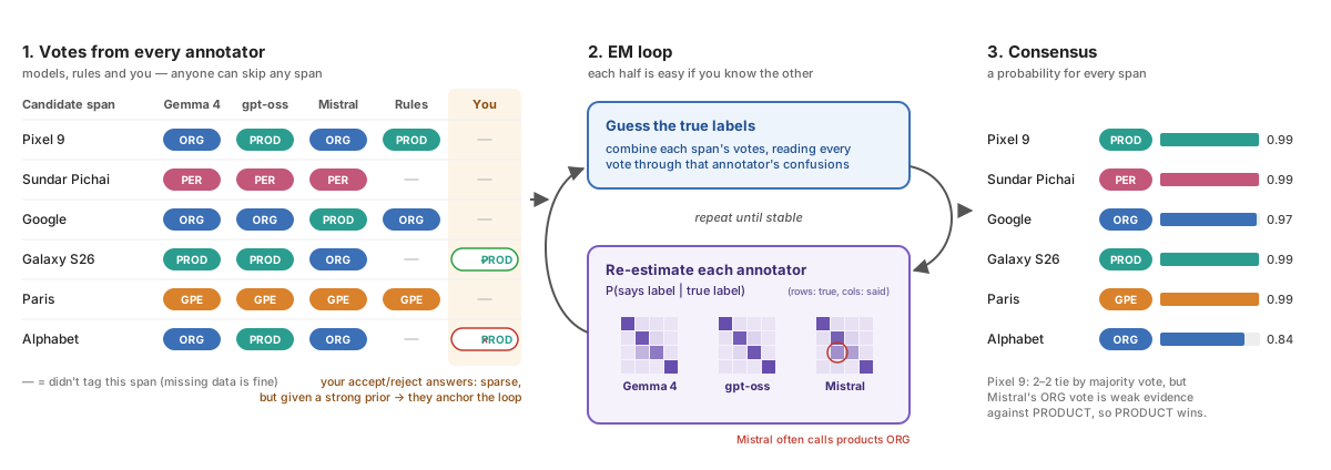
If you have annotations over the same data from five sources, how do you work out the most likely labels and how much to trust each source on average? If you knew either of those it would be easy to work out the other, so if you know neither (and you’re feeling fancy) you make a probabilistic graphical model.1
Specifically, we use Carpenter’s (2008) Bayesian adaptation of the Dawid and Skene (1979) model for annotation. Basically, you give it the category assignments from your annotators, EM goes brr, and you get back a Naive Bayes model with a × k features, where a is the number of annotators and k is the number of categories. For each instance, you run the model with its annotations as features, and you get back a probability distribution over the categories.
This is much nicer than a simple weighted voting scheme, because if an agent
frequently confuses the categories PRODUCT and BRAND, and you see it’s labeled
some item BRAND, you get to use that as partial evidence it might be PRODUCT.
In a weighted voting scheme, each annotator gets one vote, and you just figure out
how much you trust each one. In the Dawid-Skene model, each annotator can split their
vote between multiple categories, with the split determined by the category that annotator
picked.
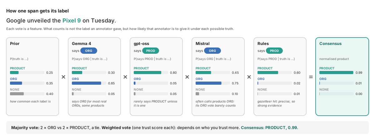
And actually, the categories predicted by the “annotators” don’t even need to be
the actual categories you want back. They’re just features. If you have a generic NER
model that predicts PER, ORG, LOC and MISC, but your actual task is to predict CANDIDATE,
PARTY and ELECTORATE, you can still include the generic NER model and see if it
helps. It might be that its LOC entities are good evidence for ELECTORATE.
The consensus model also naturally accommodates missing or partial data. You don’t need every annotator to answer every example, so you can mix in as much manual annotation as you want. We take advantage of this by setting up binary annotation tasks that a human can blitz through very quickly.
An AI-generated and minimally verified2 literature review of other uses of the Dawid-Skene model to combine agent outputs can be found in Appendix 1. The review turned up several papers evaluating Dawid-Skene on text categorization problems. The agent concluded from these papers that Dawid-Skene was beneficial when some amount of manual annotation was included in the mix. The review did not find any papers using Dawid-Skene for entity recognition.
Prompt tuning and rule-based correction
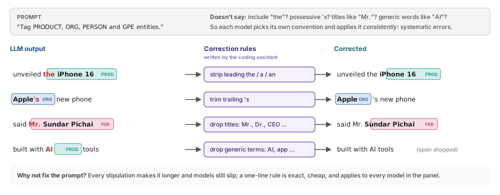
One of the challenges for zero- or few-shot entity recognition is that the task will almost always be heavily under-specified by the prompt, because there are so many details about how categories should be defined and how boundaries should be calculated. This means that agents will very often make systematic errors. We recommend letting the coding agent perform some amount of prompt tuning, but if an error can easily be addressed by post-correction rules, it’s better to do that rather than bloating the prompt with increasingly specific stipulations. The coding agent can review the agents’ outputs and implement these rules. This step can be done before or after the binary annotations, or both.
Systematic rule engineering and gazetteer construction
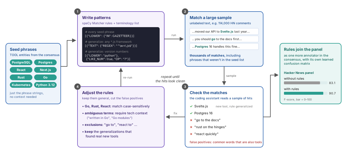
We also employ a more systematic process to create rules and terminology lists
(“gazetteers”). The coding agent is given the set of phrases labeled as entities in the data
and instructed to create rules to cover them, implemented as spaCy Matcher patterns. The agent is
then given a larger sample of unlabeled text to check and iteratively adjust the patterns,
attempting to make the rules as general as possible while minimizing the false positives.
Binary annotation
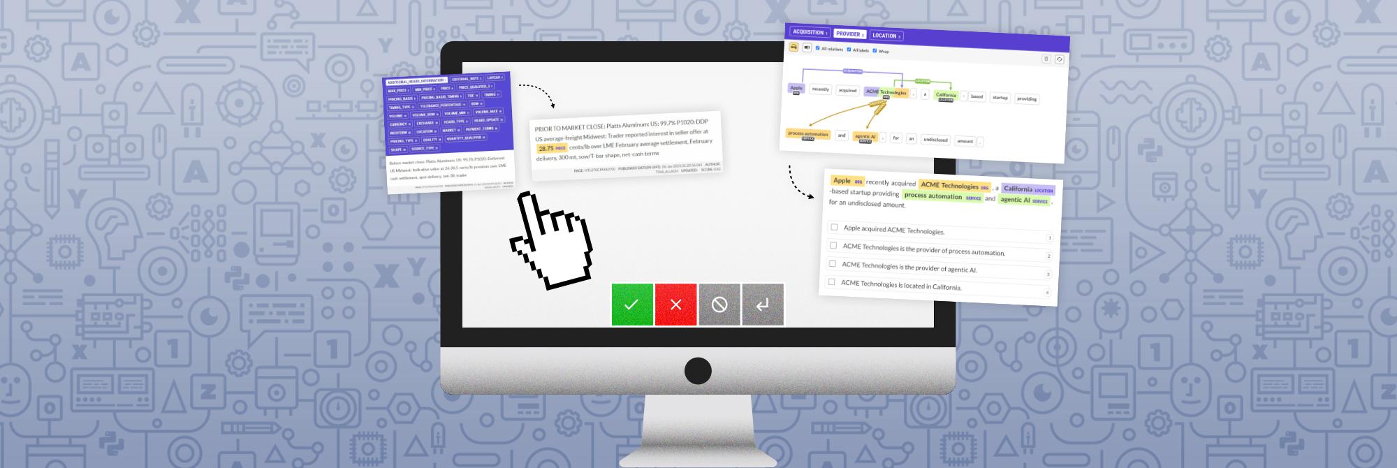
We recommend some amount of manual annotation to anchor the consensus calculation and further improve the data, and we can take advantage of the consensus algorithm to make the annotation process very efficient. In standard NER annotation, the annotator clicks and drags to highlight spans of text. Words left unhighlighted also assert an annotation in this interface, because that denotes a non-entity. This makes it hard to defer decisions, and pressures the annotator to get everything correct, because missed annotations will actively mislead the model or evaluation.
With the consensus algorithm, there’s no need for the work produced by any annotator to be complete. Missing information is no problem, because the annotator’s labels are just features in a linear model. If some feature is missing, the model can just use the others. We therefore reframe NER annotation as a binary task, of accepting or rejecting an annotation proposed by one of the agents.
In our experiments we ask only a small subset of the binary questions, focusing only on entities where the agents disagreed. This reduces the manual effort for 500 documents to around 10–20 minutes. However, even if many more questions are asked, the binary interface is fundamentally very efficient per decision. Its downside is that it cannot be guaranteed to produce a complete gold standard, because some of the correct annotations may not be presented for approval. What we gain from this trade-off is speed, which comes from three factors.
First, it’s obviously more efficient to hit a single key (or swipe on a mobile device) to accept, reject or ignore an example, instead of clicking and dragging. We even go a step further and keep the entity annotation fixed in the center of the card, to reduce eye movement.
Second, the annotation decisions can be sorted into an easier order. We use the tuple (category, phrase, confidence) as a sort key. Annotating a single category together lets you review the guidelines for that category once, and keep them in memory. Annotating occurrences of the same phrase together helps you make consistent decisions, and lets you quickly click through instances of a decision once you’ve made it, starting from prototypical (confident) cases, with less clear cases coming at the end of the run. Annotations are held in an output buffer of the client before being sent off in batches, so you can easily go back over the last few decisions if something flashed by that you want to look at.
The third reason the binary annotation is faster is that you can skip any annotation decision that isn’t immediately obvious. Entity annotations often require broad or deep knowledge, and it’s very inefficient to stop and look things up in the middle of annotation. For instance, one of our evaluation tasks consisted of entity labels over YouTube video descriptions. The descriptions could be about anything, so obviously there will be things we don’t know. The other annotators (which are AI agents) don’t need us to google these things to read an AI summary so we can cast a vote. We can just abstain.
The binary annotation also interacts positively with the consensus algorithm. The consensus algorithm has to jointly decide what the true labels are and which annotators to trust. If there are multiple low-quality annotators making the same mistakes, the consensus algorithm can start to define those incorrect annotations as the truth. The binary annotations address this, because you get annotations that you can put a high prior on, which pulls the consensus toward the truth while still allowing the possibility to be outvoted if you make a mistake. The coding assistant driving the process can prompt you or resolve these cases itself, and can set a useful prior based on the data.
Decoding
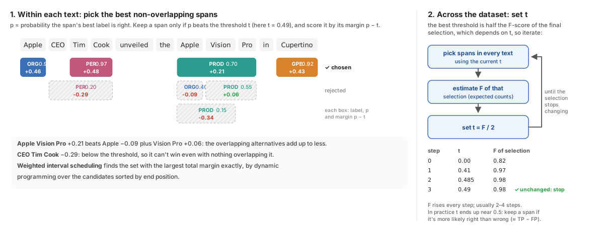
The consensus algorithm assigns every candidate span a probability distribution over the categories (with “not an entity” included as a category). The candidates can overlap, so a decoding step chooses the non-overlapping entities with the highest expected entity F-score, using Dinkelbach’s method with weighted interval scheduling (see Appendix 3).3
Experiments
| Dataset | Labels | Size | Gold |
|---|---|---|---|
| Hacker News | TOOL | 2,500 comments (100 tune, 2,000 train, 400 eval), ~45 words | 400 comments, 610 entities (165 comments with none) |
| AG News | PERSON, ORG, PRODUCT, GPE | 2,500 stories (100 tune, 2,000 train, 400 eval), ~36 words | 400 stories, 1,308 entities (ORG 701, PRODUCT 321, GPE 184, PERSON 102) |
We created two small NER datasets to evaluate our workflow.
- Hacker News (HN): Comments from Hacker News threads linking to github.com, labeled with
one entity type,
TOOL, which we defined broadly as any website, software library, language, hardware, etc. that you could compare against alternatives. We excluded formats such as JSON or Markdown, and categories of tool like “LLMs”. - AG News: Tech news snippets from the Sci/Tech class of the
AG News corpus, annotated for
PERSON,ORG,PRODUCTandGPE(geopolitical entity).ORGandPRODUCTwere often differentiated by context (e.g. “Amazon” is both a product and an organization).
The HN data is intended to stand in for entity recognition tasks that need to recognize some arbitrary but relatively simple category that isn’t recognized “off the shelf” by pretrained models such as spaCy’s NER model. An imagined context might be that you want to track relevance of different technologies, so you want to create training and evaluation data for a task-specific transformer model, as running all HN comments through an LLM will be too expensive.
The AG News task evaluates the workflow on a relatively familiar NER task, but with slightly
adjusted category definitions, and a focus on the PRODUCT category that spaCy’s models perform poorly on.
To evaluate the workflow we needed to somehow create gold standard annotations. To do this we
predicted initial entities, and then corrected them using Prodigy’s ner.manual interface, which
offers a fairly standard click-and-drag experience. This process creates annotations that are
slightly biased toward the system that was used to suggest the annotations, so for the AG News
task we performed the annotations twice, once using annotations suggested by a separate LLM
(GPT 5.6 Sol) and once
using annotations suggested by our workflow (the open-weights panel, with rules and binary
annotation corrections applied). We then did a blind resolution step for any disagreements.
For the HN gold we just started from the open-weights panel.
Which models did we use, and how did they do individually?
Our panels are built from open-weight models that each fit on a single 24 GB GPU, served with
Ollama: Gemma 4 26B-A4B (quantization-aware, with thinking turned off), gpt-oss 20B, Mistral
Small 3.2 24B and, for the AG News task, Qwen 3.8 27B (thinking off). The AG News panel also
includes spaCy’s en_core_web_trf pipeline, which predicts the standard OntoNotes categories
and so only takes part in that task. Our baseline “good LLM” is GPT 5.6 Sol.
The table shows how each annotator did on its own, before any gazetteer matching or consensus: entity-level exact-match F-score on each task’s evaluation set (400 Hacker News comments with 610 tools; 400 AG News stories with 1,308 entities). Each model’s ”+ Rules” row is the same output after the task’s correction rules (see the next section and Appendix 2), which are applied alike to every annotator.
| Annotator | Hacker News | AG News |
|---|---|---|
| GPT 5.6 Sol (baseline) | 0.871 | 0.926 |
| + Rules | 0.877 | 0.928 |
| Gemma 4 26B-A4B | 0.812 | 0.861 |
| + Rules | 0.839 | 0.879 |
| gpt-oss 20B | 0.846 | 0.852 |
| + Rules | 0.872 | 0.870 |
| Qwen 3.8 27B | 0.855 | |
| + Rules | 0.869 | |
| Mistral Small 3.2 24B | 0.706 | 0.762 |
| + Rules | 0.766 | 0.781 |
spaCy en_core_web_trf | 0.799 | |
| + Rules | 0.819 |
Correction rules and their impacts
The rules help the open-weight models by 0.01–0.06 and leave Sol nearly unchanged: they were written to fix the systematic errors the panel made, and Sol makes few of them. On Hacker News the gains come almost entirely from precision, and Mistral, the weakest model, gains the most (0.06). On AG News, where the rules also fix span boundaries, both precision and recall go up.
No open-weight model matches Sol on its own, and on AG News the gap is larger. The models also fail in different ways, which is what the consensus needs. On Hacker News, gpt-oss and Sol have the highest recall (0.90) but mark too much (precision 0.80 and 0.84), while Gemma 4 is the most precise of the panel (0.85 on Hacker News, 0.91 on AG News) and misses more. Mistral is the weakest throughout, but adding it to the AG News panel still raised the consensus F-score, from 0.889 to 0.895.
How much did the consensus help?
We ran three open-weight models over the Hacker News data, and five annotators over AG News:
- HN panel: Gemma 4, gpt-oss 20B, Mistral Small 3.2 24B,
Matcherrules - AG News panel: Gemma 4, gpt-oss 20B, Mistral Small 3.2 24B, Qwen 3.8, spaCy
en_core_web_trf
We also included a rule-based system constructed by the coding agent in the HN panel. Rules (especially a terminology list, aka a ‘gazetteer’) perform well on the HN task because tool names form a large but closed and mostly unambiguous vocabulary, which a list built from 114,000 comments covers well, and which the models individually miss in different places.
The models were run using Ollama with 4-bit weight quantization. We applied the correction rules, and then used the consensus algorithm to create a single set of annotations. We compared this consensus output to a strong commercial model (GPT 5.6 Sol) and the single best model in each panel (gpt-oss for HN, Gemma 4 for AG News).
| Annotator | Hacker News | AG News | ||||
|---|---|---|---|---|---|---|
| P | R | F | P | R | F | |
| GPT 5.6 Sol | 0.843 | 0.900 | 0.871 | 0.927 | 0.925 | 0.926 |
| Best open-weight model | 0.849 | 0.897 | 0.872 | 0.935 | 0.830 | 0.879 |
| Consensus | 0.936 | 0.880 | 0.907 | 0.944 | 0.904 | 0.923 |
The consensus outperformed GPT 5.6 Sol on the HN data, and performed similarly on AG News while being much cheaper to run (around 1/25th the price). The consensus outperformed its best contributor on both tasks. We also tried adding GPT 5.6 Sol to the panel and recomputing the consensus, but it didn’t improve results meaningfully.
The consensus algorithm has a general risk of underperforming the best model so long as no trustworthy information is included in the consensus calculation. On the HN task, a panel consisting of Gemma 4, gpt-oss 20B and Mistral scores only 0.831 F, below gpt-oss alone (0.872). Adding the rule-based system as an annotator swings the consensus to the correct annotations, taking it up to 0.907.
How much did the binary annotations help?
Our workflow includes an optional but recommended manual annotation step. The annotations are targeted to the most uncertain examples, and are presented in the highly efficient binary interface described above.
The recommended workflow is to run the panel of models, calculate the consensus, and then queue up all contested annotations as binary questions. On our data sets this generally meant a few hundred yes/no decisions, which could be completed in 10–20 minutes.
| Annotator | Hacker News | AG News | ||||
|---|---|---|---|---|---|---|
| P | R | F | P | R | F | |
| GPT 5.6 Sol | 0.843 | 0.900 | 0.871 | 0.927 | 0.925 | 0.926 |
| Consensus | 0.936 | 0.880 | 0.907 | 0.944 | 0.904 | 0.923 |
| Consensus + binary annotations | 0.945 | 0.908 | 0.926 | 0.969 | 0.940 | 0.954 |
| Binary decisions | 130 | 415 | ||||
The consensus rows are the panels from the previous section, with the correction rules (and on Hacker News the gazetteer). The binary annotations add 0.019 F on Hacker News and 0.031 on AG News, and raise both precision and recall: an accepted entity that only one or two models found is kept, and a rejected one is dropped even when most of the panel marked it. On Hacker News the gazetteer and the annotations partly fix the same misses. Without the gazetteer’s matches, the same 130 decisions take the consensus from 0.841 to 0.887.
The decisions were made on the evaluation texts themselves, so these numbers measure how much better the annotated data gets, which is the point of the workflow, rather than how well anything generalizes. The AG News gold was partly built from the panel’s reviewed output (see the gold standard above), which may favor this row slightly. The blind resolution step was there to limit that.
Annotations address a potential problem the consensus algorithm can have. If the algorithm has to bootstrap trust from scratch, it can converge on the wrong definition of the truth: the bad models can outvote the better ones. If this happens the consensus will do worse than just running the best model. Annotations solve this problem by letting the algorithm start from some trusted information. And of course, for data development, annotations help by improving the data directly.
Conclusion
Many practitioners still associate data labeling with large-scale efforts, generally involving outsourced labor. These workforces need to be “programmed” carefully, with exhaustive annotation manuals and a well-tuned task design, and you still need some quality control procedure.
Our workflow is a flexible and efficient way to create high quality span-labeled data without the overhead of engaging an outsourced workforce. For most projects a little annotation goes a long way, for both training and evaluation. You can run the workflow using our platform Ellf, which is free for solo local use.
Appendix
Appendix 1: Dawid-Skene and agent ensembles
This is a summary of a literature review Claude Code put together with research subagents. As noted above, we’ve only spot-checked it.
The classic results agree that annotator models beat majority voting when the annotators differ in quality, and make little difference when they’re uniformly good (Sheshadri and Lease, 2013; Paun et al., 2018). Snow et al. (2008) are often cited as an application of Dawid-Skene, but they estimated each worker’s confusion matrix from a small set of expert labels rather than with unsupervised EM, which is closer to what we do with the binary annotations. Passonneau and Carpenter (2014) had no gold standard, so their case is about calibrated per-item confidence and annotator diagnostics rather than accuracy over voting. They also warned that correlated annotators should widen the uncertainty.
About a dozen papers since 2023 apply Dawid-Skene or close relatives (one-coin Dawid-Skene, MACE, GLAD) to LLM labels, and the results split by who’s in the pool:
- LLMs mixed with humans: big wins. He et al. (CHI 2024) added GPT-4 as one more worker alongside an MTurk crowd. One-coin Dawid-Skene reached 87.5% accuracy, against 58.3% for majority vote and 83.6% for GPT-4 alone.
- LLMs only: ties or losses. Saïd and Villaneau (2026) ran two LLMs with three prompts each: majority vote scored 69.2%, Dawid-Skene 69.0% and the best single model 79.2%. In a three-LLM study of financial reporting compliance, Dawid-Skene and majority vote tied at 0.671 F, below the best single LLM at 0.713 (Akasukpe et al., 2026).
The problem is correlated errors. When two LLMs are both wrong, they give the same wrong answer about 60% of the time, and stronger models are more correlated, even across providers (Kim et al., 2025). Kohli (2026) estimates that a panel of nine frontier judges carries about two independent votes. Dawid-Skene assumes the annotators are independent given the true label, so it overcounts models that agree. In Saïd and Villaneau’s study it estimated one model’s accuracy at 90.7% when it was 71.0% against gold, and flagged none of 500 items as uncertain. Counting prompts or temperature samples of the same model as separate annotators makes this worse (Li, 2024).
Methods that model the dependence do better. Balasubramanian et al. (ICML 2026) fit Ising and latent-factor models over panels of ten LLM judges and beat weighted voting by 6–10 points. The strongest couplings were between models from the same provider. Ask Me Anything (Arora et al., 2023) combines prompts with a weak-supervision label model that learns the dependencies between them, gaining up to 8.7 points over majority vote. The broader LLM ensembling literature mostly finds that gains over voting come from confidence weighting or from sampling the best model more, and that multi-agent debate adds little beyond the vote (Choi et al., 2025).
The review found no papers applying Dawid-Skene to span-level tasks such as NER. Our results match the mixed-pool findings. On Hacker News the all-LLM panel scored below its best member (0.831 against 0.872). Adding the rule-based system as an annotator took it to 0.907. Without the gazetteer, 130 binary decisions took the consensus from 0.841 to 0.887.
Appendix 2: The correction rules
The coding agent wrote the rules by listing, for each agent, the phrases and labels it kept marking that the consensus disagreed with. It turned a pattern into a rule only where the annotation guidelines plainly ruled the agent’s version out, and left it alone where the guidelines didn’t settle the case or the consensus itself looked wrong. It never looked at the gold labels. Each rule records the guideline it follows, and every rule applies to every agent.
The rules run in order over each agent’s spans. Most are spaCy Matcher
patterns or phrase lists, matched on the task’s own tokens so the offsets line
up. A rule either drops a matching span, gives it another label, or cuts a
match off its start or end. A few structural rules can’t be written as a
pattern over the span alone, because they need the text around it.
YouTube
| Rule | What it does | Guideline | Example |
|---|---|---|---|
| Merge split names | Joins neighboring one-word spans with the same label | One name, one span | “Napoleon” + “Dynamite” → “Napoleon Dynamite” |
| Hashtags, handles and links | Drops spans after # or @, or inside a URL | Never mark hashtags, handles or links | “#iphone17pro” |
| Titles | Cuts “President”, “Mr.”, “Dr.” and similar off PERSON spans | Whole names without titles | “President Trump” → “Trump” |
| Places | Drops place names (13 phrases) | Places aren’t marked | “Canada”, “Texas” |
| Governments and parties | Drops them (13 phrases) | Not one of the labels | “Democrats”, “White House” |
| Events and holidays | Drops them (6 phrases) | Not one of the labels | “Diwali”, “World Cup” |
| Generic words | Drops common words and pronouns (25 phrases) | Generic words aren’t names | “golf”, “merch”, “highlights” |
| Games | Relabels to WORK | Games are works | “Minecraft”, “GTA 6” |
| Platforms | Relabels to PRODUCT | A platform you use is a PRODUCT, which comes before WORK and BRAND | “Roblox”, “YouTube” |
| Apps named after their company | Relabels BRAND to PRODUCT | A company whose app has its name is a PRODUCT | “Quince”, “LifeLock” |
| TV shows | Relabels to WORK | A TV show is a work | “SNL”, “60 Minutes” |
| Makers and outlets | Relabels PRODUCT to BRAND | No product goes by just the maker’s name; news outlets are BRAND | “Learjet”, “CNN” |
| People and characters | Relabels to PERSON | PERSON is the first label that fits | “D-Block Europe”, “Iron Man” |
AG News
| Rule | What it does | Guideline | Example |
|---|---|---|---|
| Markup | Drops spans containing HTML markup, and the font names in it | Only mentions in the story count | size=-1 color=#6f6f6f, “Verdana” |
| A leading “the” | Puts “the” inside an ORG or GPE name of several words, and leaves it out of one-word names and abbreviations; a name modifying a noun (“the Owings Mills company”) is left alone | The OntoNotes convention, which the guidelines now follow | “Department of Homeland Security” → “the Department of Homeland Security”; “the EU” → “EU” |
| “the” before products and people | Cuts a lower-case “the” off PRODUCT and PERSON spans | Only when it’s part of the title | “the iPod” → “iPod”, but “The Sims 2” stays |
| Titles | Cuts “CEO”, “Chairman”, “Dr.” and similar off PERSON spans | No titles | “CEO Steve Jobs” → “Steve Jobs” |
| Possessives | Cuts a trailing “‘s” | “‘s” isn’t part of a name | “South Korea’s” → “South Korea” |
| Nationalities | Drops them (37 phrases) | Nationalities aren’t entities | “Japanese”, “Russian” |
| Technologies and formats | Drops them (42 phrases) | Technologies, protocols, standards and formats aren’t products | “Internet”, “Wi-Fi”, “GPS”, “DVD” |
| Generic words | Drops spans made only of lower-case common words, and pronouns | Generic product types aren’t products | “cell phones”, “spyware”, “I” |
| Link labels and groups | Drops a few common words (5 phrases) | Generic words aren’t names | “Quote”, “Chart”, “Scientists” |
| Places without a government | Drops planets, moons, continents, regions, streets and oceans (24 phrases) | Only places with a government are GPE | “Saturn”, “Europe”, “Wall Street” |
| Products that are never companies | Relabels ORG, PERSON or GPE to PRODUCT (25 phrases) | Software, hardware, games, spacecraft and malware are products | “Windows”, “Firefox”, “Sasser”, “Cassini” |
| News agencies and exchanges | Relabels to ORG (9 phrases) | A news source is ORG | “AP”, “Reuters”, “Nasdaq” |
| Dateline cities | Relabels ORG, PERSON or PRODUCT to GPE (10 phrases) | Cities are GPE | “TOKYO (Reuters)” |
Phrase rules only fire on exact matches of the whole span, so “Windows” is relabeled but “Windows XP Service Pack 2” is left as it is. Rules about a company or its product (“Skype”, “PayPal”) aren’t possible, because the guidelines decide those by context.
Rules make mistakes too. The possessive rule turns “Albertson’s”, a company whose name ends in “‘s”, into “Albertson”. The pronoun pattern drops “X1”, which spaCy’s tagger mistakes for a pronoun.
Appendix 3: Decoding
The consensus algorithm gives every candidate span (any span at least one annotator marked) a probability distribution over the categories, including “not an entity”. The decoder chooses the set of non-overlapping entities with the highest expected entity F-score over the whole dataset.
We approximate the expected F-score by the ratio of the expected counts, summed over the dataset (Nan et al., 2012). Under that approximation, a span is worth predicting if its label is more likely to be right than half the F-score of the final selection (Lipton et al., 2014). So the decision is a threshold, shared by every text. Within a text, overlapping candidates compete, and weighted interval scheduling picks the non-overlapping spans with the largest total margin over the threshold.
The catch is that the threshold depends on the F-score, which depends on which spans are chosen. Dinkelbach’s (1967) method resolves the circularity by iterating: pick the spans for the current threshold, compute the F-score of that selection, set the threshold to half of it, and repeat until the selection stops changing. The F-score rises at every step, and the iteration stops at the exact optimum of the approximate objective, usually in two to four steps.
In practice the threshold ended up very close to 0.5, because the model rates its own F-score at about 0.99, well above what we measure. At 0.5 the rule is to predict a span if it’s more likely right than wrong, which is the same as optimizing TP − FP, and gave the same entities on our data.
Jansche (2007) computes the exact expected F-score instead, for models with one independent binary label per token, where spans can’t overlap.
Resources
- Ellf: Our new virtual assistant and platform for agentic NLP development
- Introducing Ellf: The missing piece for building NLP with coding assistants
- NER Data from a Panel of Open-Weight LLMs: Project template for the workflow described in this post
- Project Templates: End-to-end workflows for common NLP tasks
- Prodigy: A modern annotation tool for NLP and machine learning
- Named Entity Recognition with Prodigy: Documentation and workflows
- A practical guide to human-in-the-loop distillation: How to distill LLMs into smaller, faster, private and more accurate components
Bibliography bibliography
- IFRS Compliance Verification: An Open Multi-LLM Benchmark and Content-Conditioned Ensemble Classifier (Akasukpe et al., 2026)
- Ask Me Anything: A Simple Strategy for Prompting Language Models (Arora et al., 2023)
- Dependence-Aware Label Aggregation for LLM-as-a-Judge via Ising Models (Balasubramanian et al., 2026)
- Multilevel Bayesian Models of Categorical Data Annotation (Carpenter, 2008)
- Debate or Vote: Which Yields Better Decisions in Multi-Agent Large Language Models? (Choi et al., 2025)
- Maximum Likelihood Estimation of Observer Error-Rates Using the EM Algorithm (Dawid and Skene, 1979)
- On Nonlinear Fractional Programming (Dinkelbach, 1967)
- If in a Crowdsourced Data Annotation Pipeline, a GPT-4 (He et al., 2024)
- Learning Whom to Trust with MACE (Hovy et al., 2013)
- A Maximum Expected Utility Framework for Binary Sequence Labeling (Jansche, 2007)
- Correlated Errors in Large Language Models (Kim et al., 2025)
- Nine Judges, Two Effective Votes: Correlated Errors Undermine LLM Evaluation Panels (Kohli, 2026)
- A Comparative Study on Annotation Quality of Crowdsourcing and LLM via Label Aggregation (Li, 2024)
- Thresholding Classifiers to Maximize F1 Score (Lipton et al., 2014)
- Optimizing F-measure: A Tale of Two Approaches (Nan et al., 2012)
- The Benefits of a Model of Annotation (Passonneau and Carpenter, 2014)
- Comparing Bayesian Models of Annotation (Paun et al., 2018)
- Multi-Source Emotion Annotation in Children’s Language: When LLM Consensus Diverges from Human Judgment (Saïd and Villaneau, 2026)
- SQUARE: A Benchmark for Research on Computing Crowd Consensus (Sheshadri and Lease, 2013)
- Cheap and Fast — But is it Good? Evaluating Non-Expert Annotations for Natural Language Tasks (Snow et al., 2008)
- Whose Vote Should Count More: Optimal Integration of Labels from Labelers of Unknown Expertise (Whitehill et al., 2009)
Footnotes
-
I realize this won’t make much sense if you don’t already know what a probabilistic graphical model is. If you paste these paragraphs into Claude or ChatGPT you’ll get an explanation that meets you where you are, which is better than I can do.
-
We clicked on the links and flicked through them a bit, but didn’t read the papers properly.
-
This bit of optimization was an interesting but inconsequential win for our coding agent, Claude Code (running Opus 5.5). F-measure is tricky to use in decoding because it’s not incremental. In spaCy we settle for optimizing TP − FP, which approximates F-score well enough as a figure-of-merit and works easily in the greedy parser’s imitation learning objective. When instructed to implement a decoder optimizing for F-score, Claude Code found some of the relevant papers, but implemented a solution using a fractional programming technique (Dinkelbach’s method) that is not well known in NLP as far as we’re aware. The technique made no difference over TP − FP on these experiments, but we kept it in because we found the detail charming.