
- 34 minute read
- Blog
- spaCy
- Coreference Resolution


Coreference resolution is something all of us do instinctively many times every day even though most of us haven’t heard the term before. People use language to talk about entities, events and the relationships between them. When we mention the same thing multiple times throughout a discourse we tend to use different expressions. For example:
Here “the bass” and “it” refer to the same entity. Within natural language processing, coreference resolution is a core task that helps with a large array of tasks ranging from machine translation all the way to information extraction. In this post we will introduce spaCy’s new CoreferenceResolver and SpanResolver components and show how they can be assembled into an end-to-end coreference resolution pipeline!
What is coreference
To understand coreference, consider a fictional story populated by various characters who, throughout the story, appear in various locations and face a variety of situations, as well as each other. The narrator refers to these characters, places and events in all sorts of ways. Similarly, authors of news articles, restaurant reviews or scientific articles refer to various different kinds of buildings, festivals, drug treatments and much more. Our everyday discourse with colleagues, friends and family is comprised of mentioning various things and then referring back to those things in a different way at a later time.
When an entity or an event has already been introduced in the discourse and we mention it later, that’s called coreference. In other words, when two expressions refer to the same thing, we say that they corefer.
Most of the time we do not want to keep repeating ourselves. Compare this:
Sarah enjoys a nice cup of tea in the morning. Sarah likes the cup of tea with sugar and a drop of milk.
with something like this:
Sarah enjoys a nice cup of tea in the morning. She likes it with sugar and a drop of milk.
The second one is much nicer, wouldn’t you agree? Here we used pronouns “she” and “it” to make the text more fluent.
The referents considered in practical coreference systems are more typically objects and people rather than events, and so the focus is more on nouns rather than verbs. Even though systems for event-coreference exist and have practical relevance, the most common use cases in English are resolving the referents of pronouns to noun phrases.
For example consider the discourse:
Alice 😌 practiced with her new violin 🎻 yesterday for the first time. She 😌 fell in love with the instrument 🎻 immediately, it seems like she 😌 has finally found the one 🎻.
Here “her”, “She” and “she” refer to “Alice”, while “the instrument” and “the one” refer to the “violin”. From this example alone we can already see that we are trying to solve a sort of clustering problem.
A Tricky Problem: Split Antecedents
More precisely the problem is treated as a clustering problem over non-overlapping spans in a document. The non-overlapping constraint renders the system incapable of handling the “split antecedent” problem. For example in “Alice and Bob said they like cheese, but he prefers sushi.” The pronoun “they” refers to “Alice and Bob” and “he” refers to “Bob”. However, the span “Bob” is inside “Alice and Bob” so we have to choose to either resolve “they” to “Alice and Bob” or “he” to “Bob”. The lack of split antecedent handling is a limitation of many coreference resolutions systems including ours.
We have two clusters
- 😌: (Alice, her, She, she)
- 🎻: (violin, the instrument, the one).
A coreference resolution system needs to look for mentions of entities and then try to cluster the mentions of the same entity together. Each mention is a span of text, i.e. a contiguous sequence of words. Systems learn from gold standard annotations, which group these spans into entity clusters. The clustering is evaluated by comparing the grouping of mentions produced by the system to the ground truth clustering provided in the test data.
Neural coreference resolution
The coreference resolution system we released in spacy-experimental v0.6.0 is an end-to-end neural system applicable across a wide variety of entity coreference problems. Let us walk through a really quick history to share the reasoning behind our choice of architecture for this release.
The fully deep-learning-based paradigm of coreference resolution systems starts with the paper End-to-end Neural Coreference Resolution written by Kenton Lee, Luheng He, Mike Lewis and Luke Zettlemoyer in 2017. The systems in this paradigm share the design choice of abandoning the use of pre-trained parsers, mention detectors and other learned or rule-based components during training and inference.
Following Lee et al. (2017), most systems in the neural paradigm are span-based: they produce pairwise coreference scores between contiguous sequences of tokens indicating how likely is it that they belong to the same cluster.
Since 2017 the field has seen a significant increase in performance, mainly due to the introduction of large pre-trained transformer models. The mighty BERT was introduced into the field of coreference resolution in the article BERT for Coreference Resolution: Baselines and Analysis by Mandar Joshi, Omer Levy, Luke Zettlemoyer and Daniel Weld (Joshi et al., 2019). The performance was improved a little bit by the introduction of the SpanBERT pre-trained transformer that — as the name suggests — was developed to support the learning of span features.
From span-level to word-level
Before delving into the details of these systems let’s just agree that span scoring is costly. For a document with N words we have (N(N+1))/2 number of spans. This is 5050 spans for a document with 100 words growing to 20,100 for a document with 200 words 🤯. Here is some example code extracting all spans to give you some intuition:
text = "Let's extract some spans from this sentence right here!"tokens = text.split()spans = []for n in range(1, len(tokens) + 1): for start in range(len(tokens) - (n - 1)): spans.append(tokens[start:start + n])Using the big O notation we drop the constants and get O(N^2) spans, which gives us a O(N^4) complexity when scoring all possible pairs:
scores = []for i in spans: for j in spans: scores.append(score(i, j))To be fair most systems are trying to find antecedents for mentions, meaning for each span we only consider preceding spans:
scores = []for i in range(0, len(spans) - 1): for j in range(i, len(spans)): scores.append(score(i, j))… but still 😒.
It’s not crucial for us to understand the following in detail here, but it’s interesting to note that to sift through this combinatorial haystack Lee et al. (2017) already considered a list of tricks to make it somehow tractable:
- Limit the size of the spans to some maximum length.
- Consider spans only within a certain distance.
- A cheap function that assigns a score to each span indicating how likely it is that it’s a mention in general.
Both points 1. and 2. reflect our intuitive notions about coreference: there should be a reasonably small number of tokens that we would consider belonging together forming a mention and it’s unlikely to refer back to very distant parts of the text due to human working memory limitations. All of this sounds pretty reasonable, however, there are a bunch of hidden implementation details and sneaky hyperparameters lurking in there.
A year later in 2018 another influential paper from the same group titled Higher-Order Coreference Resolution with Coarse-to-Fine Inference introduces yet another component that produces cheaper pairwise “coarse” scores. These coarse scores are then used for a further pruning step before doing the more expensive calculations. Basically, as long as we are doing pairwise span-scoring we have to add modeling and code complexity in order to reduce runtime and space complexity.
To avoid these problems entirely, we’ve based our implementation on a recent incarnation of the neural paradigm published in the paper Word-Level Coreference Resolution by Vladimir Dobrovolskii, which was published in EMNLP 2021. Thank you for your work Vladimir! As the title suggests we sail from the vast oceans of scoring all spans in O(N^4) time towards the gentle seas of O(N^2) comparisons on the word level. The architecture is composed of two components: a CoreferenceResolver that clusters on the level of tokens and a SpanResolver that reconstructs the spans around each token in the clusters.
From spans to heads
First things first: training data generation. As explained our approach is word-level, but all the annotations are on the span-level. This means that we’ll need to somehow choose the single “most important” token from each span during training. Hopefully one that will allow us to reconstruct the full span in a later step. Let’s take an example:
The light of the lava lamp deepens my experience of my environment. It transforms the room into a peaceful refuge.
What are we referring to here? So we have “my”, which is basically me the speaker — hello there — but also the “the light of the lava lamp” to which “it” refers back to. Also, “the room” and “peaceful refuge” are referring to “my environment”. We have two clusters:
- The light of the lava lamp, It
- my environment, the room, a peaceful refuge
Now, which single words are we going to pick for each span? Let us run the transformer-based English pipeline called en_core_web_trfand plot the dependency tree for the first sentence with displacy.
import spacyfrom spacy import displacy
nlp = spacy.load("en_core_web_trf")doc = nlp("The light of the lava lamp deepens my experience of my environment.")displacy.serve(doc, style="dep")
Which token should we pick as the head of the span “the light of the lava lamp?” The definition of the head of the span that we use is this: the word whose head is outside of the span or is the root of the sentence is the head of the span.
The span “the light of the lava lamp” is headed by “light”: it is not connected to any of the words in the span, rather, it is directly connected to the root “deepens” and is the head of the noun-subject nsubj of the sentence.

Let’s now check “peaceful refuge”: “refuge” is the pobj (prepositional object) of “into” and “into” is outside of the span so we pick “refuge” as the head.
That’s it! It is pretty convenient that spaCy already implements the solution for this problem and for each span we can get the head with span.root:
nlp = spacy.load("en_core_web_trf")doc = nlp("It transforms the room into a peaceful refuge.")doc[-3:-1]>>> peaceful refugedoc[-3:-1].root>>> refugeBut hang on a minute, the whole point was that we move from span-level to word-level for efficiency, but what about runtime of the dependency parser? Well the good thing is that we only really need it to generate the training data, but during training and prediction we won’t need it anymore!
Coreferent scoring
The first neural module in the coreference resolution pipeline is responsible for producing a score between pairs of words indicating how likely it is that one is the antecedent of the other i.e.: how likely it is that a previous word corefers with a later one.
Let us take a very simple one-sentence example here to illustrate the process:
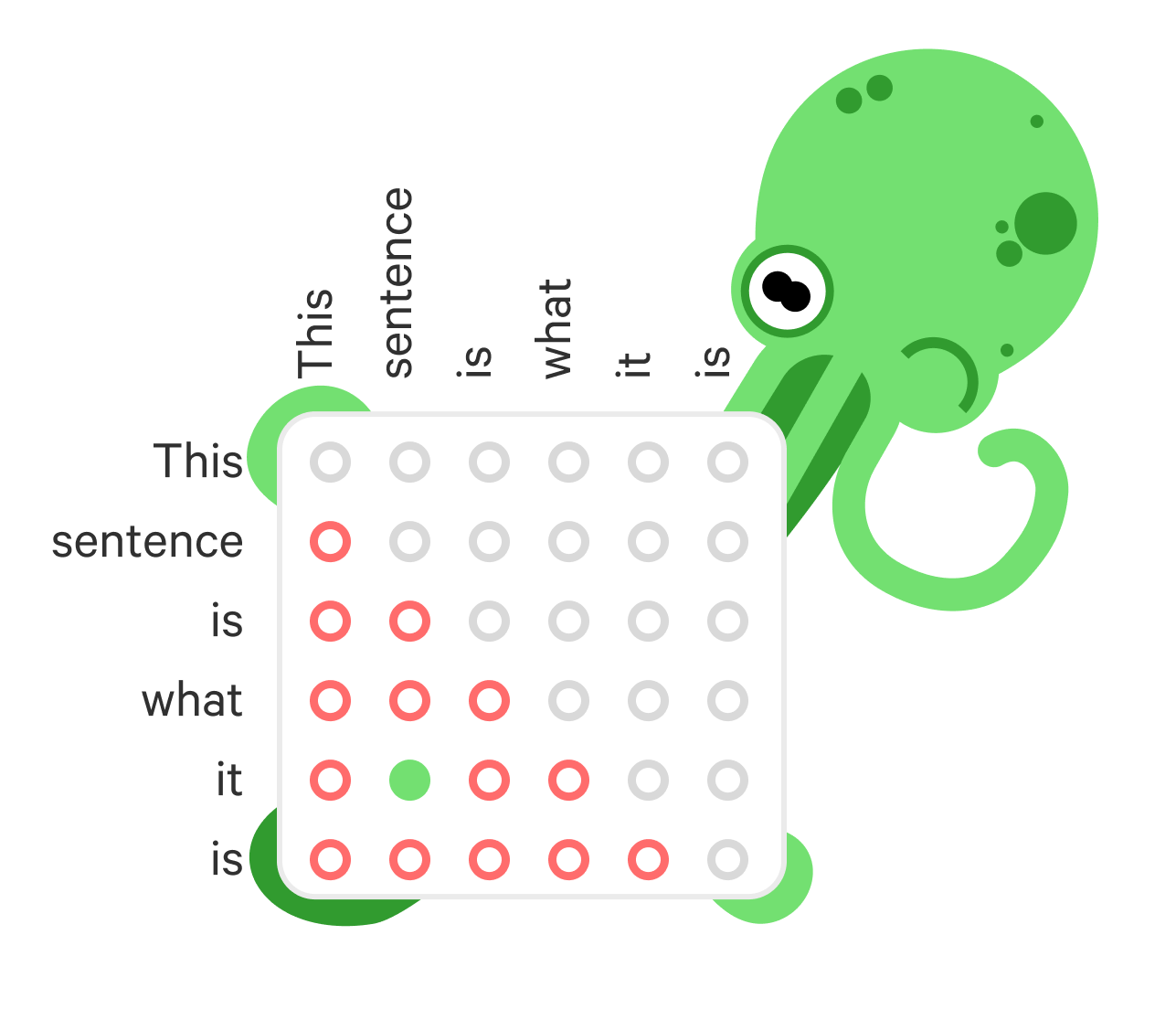
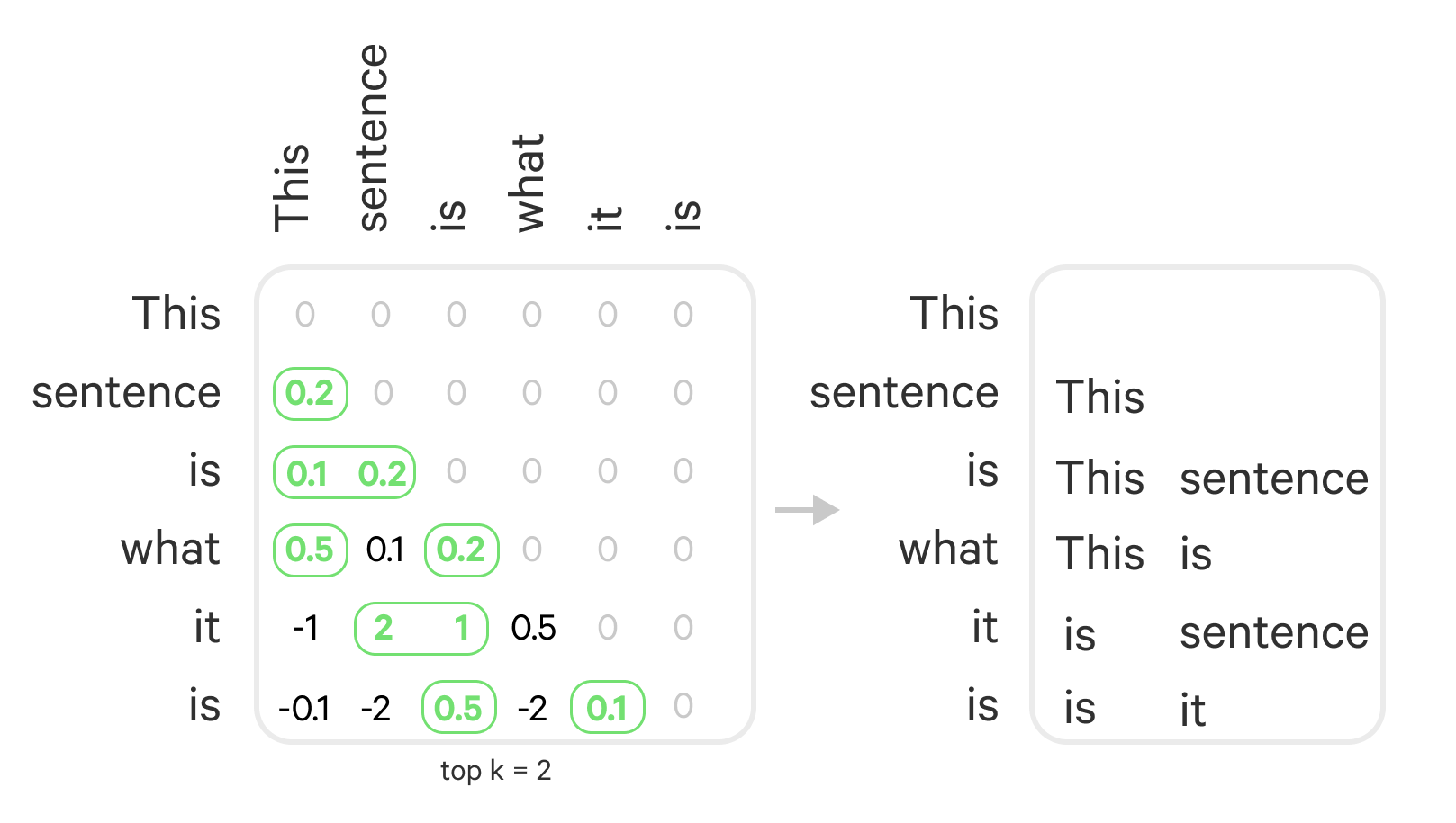
Take this sentence as just literally what it is.
Here we have “it” referring to the span “this sentence” whose head is “sentence”. Now for each word we will output a score that describes how likely it is for each previous word to be its antecedent. For demonstration let’s use (hollow) red circles to indicate a “no” decision and (filled) green circles to indicate the argmax. The grey circles are placed in cells of word pairs we do not consider because we only score each pair once. We also fill the diagonal with grey circles since a token cannot be its own antecedent.
To get these scores we perform the steps illustrated on the figure below. Let us move from this matrix representation to the perhaps more natural graph representation of the problem. We will think of the sentence as a graph where each node is a token and each edge is a potential relation between them.
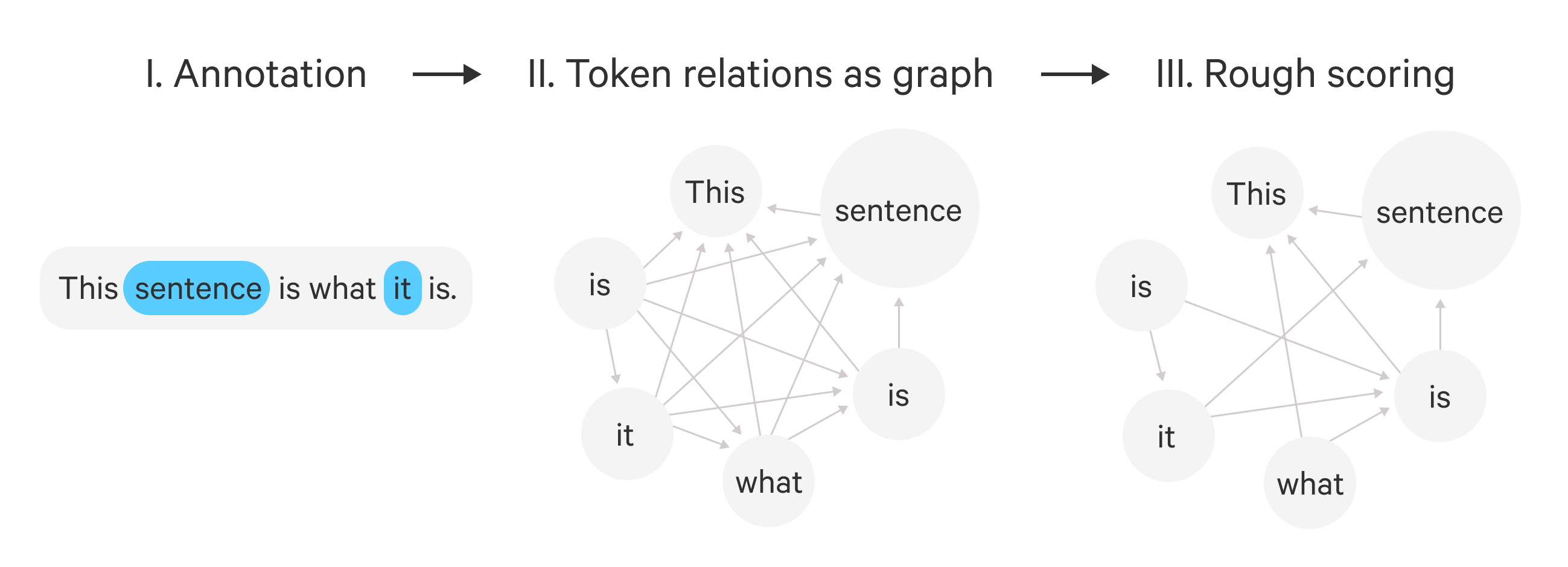
- First we assume any token could be related to any prior token.
- Then the rough-scorer keeps only the most likely coreferents for each token. It computes all pairwise scores and applies the
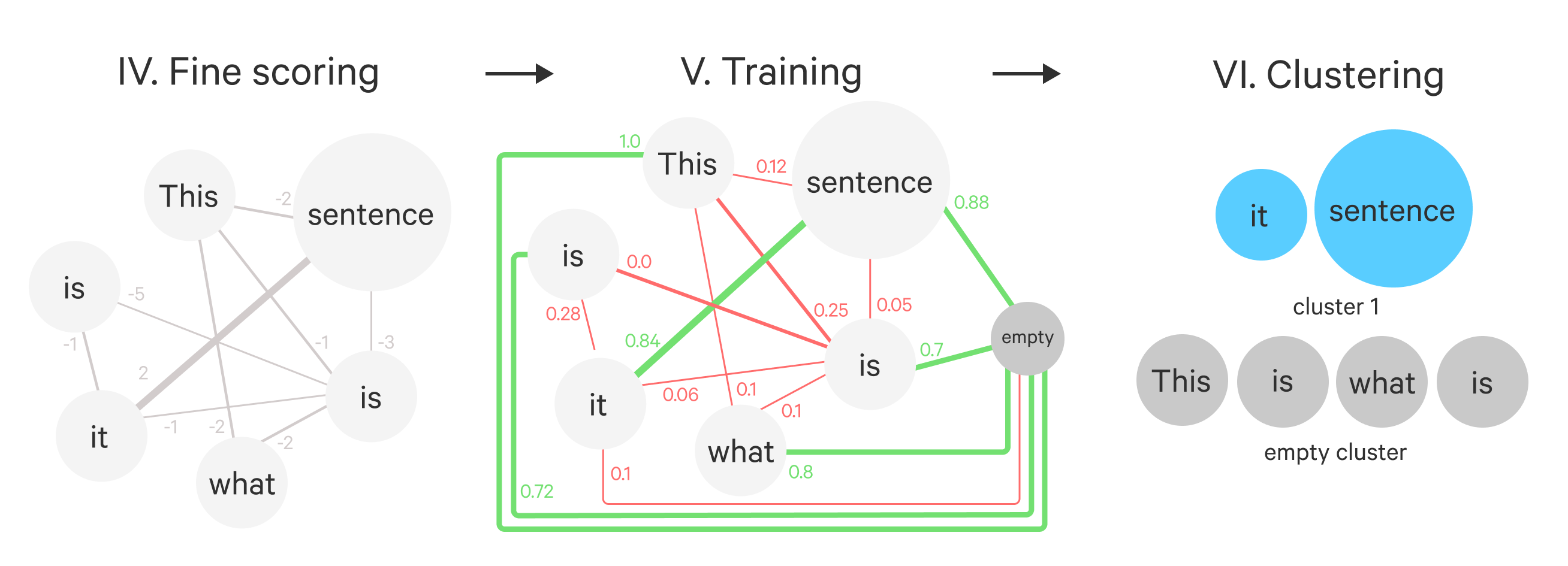
topkoperation to them to retain the pairs with the highest scores. It returns the sparsetopk-graph. - The fine-scorer takes the sparsified graph and places a weight on each edge indicating how likely two words are to corefer. It returns the weighted version of the
topk-graph. - We place the special empty node in the graph and connect it with weight 0 to all other nodes. We will use this node to absorb all tokens that are not part of any cluster.
- During training we normalize the edge-weights with
softmaxin such a way that the sum of edge weights add up to 1 for each node. We use this normalizedsoftmax- graph and the corresponding labels for training. - During inference we compute the
argmaxgraph instead: for each node we keep the largest outgoing edge. This disconnects the graph and we take the resulting connected components as the clusters. Nodes that ended up in theemptycluster are not returned by the component.
To prune the graph we use topk, to normalize the edge-weights we use softmax and to infer the best clustering we use argmax. All these operations are applied node-wise.
Tokens to vectors
To get going we need to extract features from the documents. For the coreference pipeline we use a transformer component in place of the leaner tok2vec to get better performance. Specifically, we build on the RoBERTa base which first chops up the text into subword units, then spacy-transformers aligns these subwords with the tokens produced by the tokenizer. This is done by pooling the word-pieces together. We run an additional LSTM over the RoBERTa features as we saw improvements from this extra step of processing.
Rough scores
The goal of this layer is to keep only the top-k most promising antecedents for each token. It is implemented as a cheap bilinear scoring function between all pairs of tokens.

As we discussed in the beginning when we have a document of n words we have n^2 pairs so the complexity of the CoreferenceResolver is O(n^2). The goal of the rough-scorer is to reduce the number of pairs to n * k rendering the complexity of the downstream component O(n). What the rough-scorer layer is doing is to take a fully connected graph of all token-pairs and for each node only keep k edges.
In the example below we have two tokens 🐟 and 🐡 represented by two 96 dimensional vectors and W is the learned parameter matrix:
d = 96🐟 = numpy.random.random((d, )) # vector of length d🐡 = numpy.random.random((d, )) # vector of length dW = numpy.random.random((d, d)) # d x d matrixscore = 🐟 @ W @ 🐡 # x @ y is numpy.dot(x, y)# often implemented like the line below# with a linear layer: linear(🐡).gemm(🐟)🐟 @ W @ 🐡 == W @ 🐡 @ 🐟>>> TrueWe can also compute all pairwise scores in one shot. In the example below we have a document with 113 words:
X = numpy.random.random((113, 96))S = X @ W @ X.TS.shape>>> (113, 113)Here we stored all pairwise scores in the matrix S. To only consider each pair once, we mask the matrix such that each token is only connected to preceding tokens. For example with numpy we can do:
numpy.ones((5, 5))>>>array([[1., 1., 1., 1., 1.],       [1., 1., 1., 1., 1.],       [1., 1., 1., 1., 1.],       [1., 1., 1., 1., 1.],       [1., 1., 1., 1., 1.]])
numpy.tril(np.ones((5, 5)), k=-1)>>>array([[0., 0., 0., 0., 0.],       [1., 0., 0., 0., 0.],       [1., 1., 0., 0., 0.],       [1., 1., 1., 0., 0.],       [1., 1., 1., 1., 0.]])
Here tril stands for “lower-triangular” which starts from the bottom left corner of the matrix and goes up until the diagonal. The k=-1 means that we move the diagonal down-left one step so that there are more 0s than 1s. This is because a token cannot be its own coreferent. The full code to get the rough-scores with a single bilinear function with masking is something like:
S = numpy.tril(X @ W @ X.T, k=-1)Finally, the main reason we are doing this is to prune: for each token we are only going to keep for each token its k most likely antecedents.
In the example below for each row we pick the top 3 columns, which would correspond to taking the top 3 highest scoring antecedents for each token. In PyTorch this is implemented as :
scores = np.random.randint(0, 10, (5, 6))S>>>array([[5, 1, 9, 7, 0, 0],       [7, 0, 1, 2, 8, 0],       [9, 6, 2, 3, 9, 2],       [8, 5, 6, 7, 4, 6],       [1, 8, 1, 7, 1, 3]])
scores = torch.tensor(scores)top, which = torch.topk(scores, k=3)top>>>tensor([[9, 7, 5],        [8, 7, 2],        [9, 9, 6],        [8, 7, 6],        [8, 7, 3]])which>>>tensor([[2, 3, 0],        [4, 0, 3],        [4, 0, 1],        [0, 3, 5],        [1, 3, 5]])
torch.gather(scores, 1, which) == top>>>tensor([[True, True, True],        [True, True, True],        [True, True, True],        [True, True, True],        [True, True, True]]).
Fine scores
After pruning with the bilinear rough-scorer the system allocates more resources to score the most promising candidate pairs. The goal of the fine-scorer is to take the graph produced by the rough-scorer and place weights on each edge that is proportional to the likelihood that the two tokens corefer.
The architecture of the fine-scorer is a simple multilayer network:
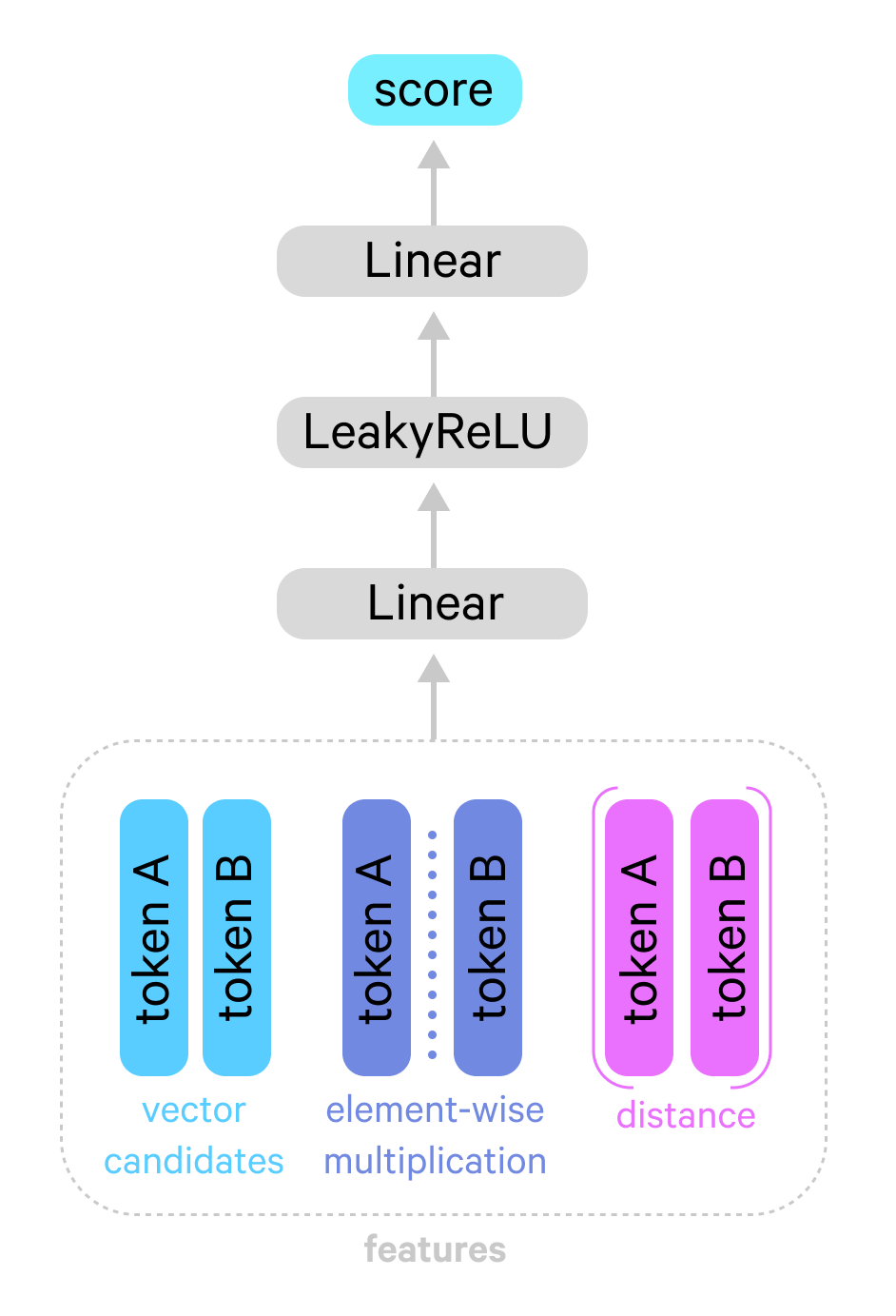
The input in this case is a matrix where each row corresponds to the pairwise features between two candidates. The feature vector used in the CoreferenceResolver is a concatenation of:
- The vector for the candidate token
🐟 - The vector for the candidate antecedent
🐡 - Their element-wise multiplication:
🐟 * 🐡 - An embedding of their linear distance:
D(🐟, 🐡)
So each row of the matrix X will become [🐟; 🐡; 🐟 * 🐡; D(🐟, 🐡)]
Intuitively it’s a fair prior assumption that the closer two tokens are the more likely it is that they corefer. But how do we use the distance between two tokens as a feature? We use a coarse way of representing distances: we take the natural logarithm of the distance between tokens and round it to the closest integer. This is how the log function transforms the distances:
log(2.71) ~= 1, log(7.38) ~= 2, log(20.08) ~= 3log(54.59) ~= 4, log(148.41) ~= 5, log(403.42) ~= 6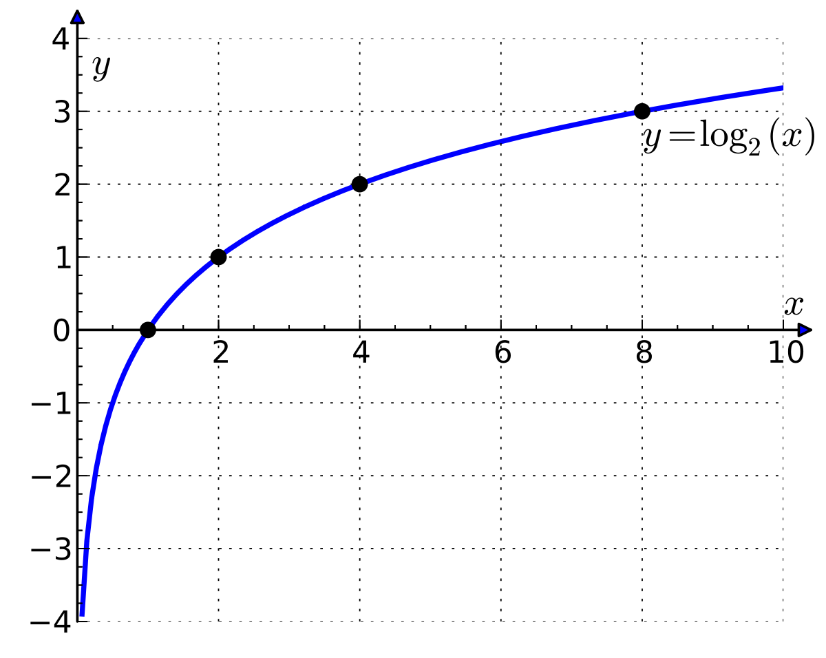
From the graph of log(x) it’s clear that it kind of “tames” the growth: as x increases, y = log(x) increases exponentially more slowly i.e.: x = log(exp(x))
The resulting integer is used as an index to an embedding table:
import numpyfrom math import log
def get_distance(i: int, j: int) -> float:    return round(max(0, log(j - i)))
num_dist = 6d = 30D = numpy.random.random(num_dist + 1, d)🐟 = 28🐡 = 357dist = get_distance(🐟, 🐡)D(🐟, 🐡) = D[min(num_dist, dist)]
Here we used D as the embedding table for the distances. We consider six distance buckets plus one for “long” i.e.: distances longer than we handle 😓. The resulting distance embedding is concatenated with the feature vectors and used in the score computation. The fine-scorer takes these features and maps them to a single number indicating how likely is it that the two tokens corefer: fine-scorer([🐟; 🐡; 🐟 * 🐡; D(🐟, 🐡)]) -> 12.3 for example. These scores will be normalized into probabilities later for the loss computation.
So why is this component more expensive? Well, the bilinear rough-scoring layer consisted of a single d x d matrix. For the dimensionality of 768 — the size of the RoBERTa base model used in the pipeline — this is 768 * 768 = 589824 parameters. Now let’s calculate how many parameters we would need for the Linear(LeakyReLU(Linear(X))) architecture. Let’s say we set the hidden dimension to a modest 256. In this case the input layer has the size (768 + 768 + 768 + 30) * 256, where 30 is the distance embedding size. This comes out to be 597504. For the second layer of computation we have only a vector of 256 * 1 to compute the scores, which adds up to 597504 + 256 = 597760. Almost the same as the bilinear. For better accuracy, however, we use a hidden size of 1024 by default giving us 2391040 parameters, which is four times as much as a rough scoring layer.
The fine-scorer also requires more space due to the explicit allocation of pair representations. Let us define two matrices A and B both of size n x d and let W be a d x d matrix. The bilinear scorer allocates a new matrix W @ A first and then multiplies the result with B. The size of this temporary matrix is n x d. For the fine-scorer, however, we need both vectors and their elementwise multiplication concatenated which is n x 3d plus the size of the distance embedding, which is why it ends up relatively large.
Loss computation
The final moving part to get the CoreferenceResolver going is to define some sort of loss function that permits gradient-based optimization. Just to reiterate: we chose an approach that treats coreference-resolution as a supervised clustering problem. As such neither the training data nor the loss function is the kind we are used to from classification or regression problems.
As in most deep learning methods today the trainable spaCy components almost always use the cross entropy loss function. During optimization we are trying to maximize the probability of some sort of category, which turns out to be the same as minimizing the negative log-likelihood of that category.
Usually in practice this means that a neural network takes some data and runs a bunch of differentiable operations one after the other. The very last operation gives us a vector of scores s , which we often call “logits” indicating how relevant each category is to the data point. Then we run the function softmax(s) to project the unconstrained scores s onto the probability simplex, which is just a fancy way of saying we normalize the scores to form a categorical distribution i.e.: they become values between 0 and 1 and sum to 1.
import numpy
def safe_softmax(x):    exp_x = numpy.exp(x - numpy.max(x))    return exp_x / exp_x.sum(axis=0)
n_samples = 9n_classes = 3S = numpy.random.random((n_samples, n_classes))  # matrix of scoresprobs = safe_softmax(s)  # matrix of probabilitiesprobs.sum(axis=0)>>> array([1., 1., 1., 1., 1., 1., 1., 1., 1.])
The softmax above is a “safe” version in that we subtract the maximum value from the logits to avoid blowing up the result of the exponentiation. This is how it’s practically implemented instead of the original exp(x) / exp(x).sum(axis=0) formulation, but they give the same result.
Components in spaCy produce categories on different levels: textcat predicts on the document-level, spancat on the span-level and tagger on the token-level. Through the softmax transformation all these models produce some probability p_c for the correct category c and we are aiming to minimize -log(p_c) meaning we are maximizing p_c. Since probabilities add up to 1 when we are pushing the probability of the right thing upwards ✔️ 👆 we are also pushing down on the probabilities of the wrong categories ✖️ 👇.
So what should these target categories be for coreference resolution? What we are aiming to do is to cluster tokens together. For each token then we should have a single cluster-id as target: each token either belongs to one of the entity-clusters or to the special empty cluster. If we had such annotation we could maximize the probability of the tokens belonging to these clusters and we arrive to a nice classification problem. However, … what would this even mean? For each document we have different clusters so we have no notion of a fixed set of target categories like we have in the usual classification problems.
We could go down another route if we had a single correct antecedent for each token and try to maximize the probability of these relationships one by one. Unfortunately we don’t even have that since there is no single target token for each token and we only have the entity-clusters which are groups of tokens. For each token we know what the other tokens are that belong to the same cluster, but that’s it. This is all we have, so how do we make use of it? How do we frame a learning problem where the model has to make a particular choice for each document, but the options vary per document?
First of all we are going to use the softmax function to normalize all the pairwise scores we computed with the fine scorer between tokens j and potential antecedents i resulting in a vector of probabilities p. In other words we normalize the edge weights so that they sum to 1 for each node.
For each tokenj we know which tokens i belong together with them in the same cluster. So now we can just go ahead and sum the components of p that correspond to tokens that are in the same cluster as j. This is the same as saying that we sum the weights of the correct edges in the graph.
This will allow us to push up ✔️ 👆 the scores between the tokens that belong to the same cluster and push down ✖️ 👇 otherwise. Even though we don’t have a single target we have multiple equally important targets: for each token all other tokens in the same cluster are together the target! In code this is something like:
import numpy
antecedent_probs = numpy.array(    [       0.08795488, 0.02744246, 0.08956143, 0.04418612, 0.03252369,       0.03073252, 0.1039334 , 0.04270362, 0.01031098, 0.03042277,       0.0846247 , 0.0552805 , 0.00247768, 0.09231465, 0.05495827,       0.03030049, 0.08119993, 0.02194266, 0.01888707, 0.05824214    ])same_cluster = numpy.random.randint(0, 19, (4,))same_cluster>>> array([ 7,  4,  8, 16])antecedent_probs[same_cluster]>>> array([0.04270362, 0.03252369, 0.01031098, 0.08119993])antecedent_probs[same_cluster].sum()>>> 0.16673822587187803
The clustering loss is a really cool idea, because it reuses the familiar softmax + cross entropy machinery with only a slight change, which gives us an end-to-end trainable coreference model that is not too different from other spaCy components.
The empty cluster trick
The final piece in the puzzle is how to set the target for the vast majority of tokens that do not appear in any cluster? Similarly, when we are actually predicting the entity clusters how are we going to say that “token i belongs to none of the clusters”? This issue is solved by simply adding an extra vector filled with 0 to the scores coming from the fine-scorer. The special 0 is added for all tokens, including the ones that appear in entity clusters. This means that, by definition, all tokens have a score of exactly 0 for belonging to the special empty cluster. During training we set the empty cluster as the target for tokens that do not belong to any cluster and let the model learn around this default: scores less than or equal to zero mean empty cluster and positive scores mean entity cluster predictions.
Inferring clusters
Not only do we need to be creative with our loss function, but we also have to do a bit of non-trivial work to find the final clustering. When we are predicting a single category per document, prediction is easy. During training we use softmax(s) to normalize the scores for the loss computation and during testing we call argmax(s) to pick the category with the highest score. However, a common situation within NLP is that rather than looking for a single category we are looking for some sort of structured object. When we are looking for parse trees, semantic graphs or in our case a clustering, we end up with a system that interleaves different kinds of search algorithms and learning components.
So far we described a model that is trained in such a way that it should output for each token 🐟 higher scores for tokens 🐡 that appear in the same cluster compared to the ones that do not 🐚. Basically, at this point all we have are pairwise scores, but what we want are clusters.
The CoreferenceResolver in spaCy uses an efficient first-order greedy inference strategy where for each token 🐟 we pick the highest scoring token 🐡 as its predicted antecedent. Doing this for all tokens gives us a disconnected graph where tokens i are interpreted as nodes of the graph and antecedent relationships are interpreted as edges (i, j). Performing breadth-first search on this disconnected graph gives us the connected components, which are the resulting final clusters. The component of the graph that would correspond to the empty cluster is not included in the output.
By first-order we mean that when making decisions we are being very local: for each token 🐟 we pick the best antecedent 🐡 independently and we are neither basing our future decisions on previous decisions nor are we considering pairs or triples of decisions at a time. While this sounds like a real bummer it turns out that in practice higher-order inference does not add too much, and even if it does it’s not in a reliable fashion.
Just a final note here. We’ve discussed before that we block out the scores for pairs of tokens where j >= i, because the model only considers referring backwards, but not referring forwards. But since the final predictions are clusters the precedence in the linear order of document does not matter. Consider the sentence:
After he sat in the car, Peter turned on the engine.
Here “he” refers forward to “Peter”. The model never produces a score for the pair [he, Peter], but it does produce a score for [Peter, he] which means that the inference algorithm will place these two spans in the same cluster anyhow.
Span resolution
So far we were in the land of tokens, but we would like the final prediction to be on the span level. For example in:
The beautiful octopus dreams of itself finding a gigantic coral reef.
We would like to infer that “itself” and “the beautiful octopus” belong to the same cluster. Rather than simply returning “octopus” we would like the whole noun-phrase “the beautiful octopus”. The job of the SpanResolver is to take the token “octopus” and predict that the token “the” is the start of the span and the token “octopus” is the end of the span that is headed by “octopus”.
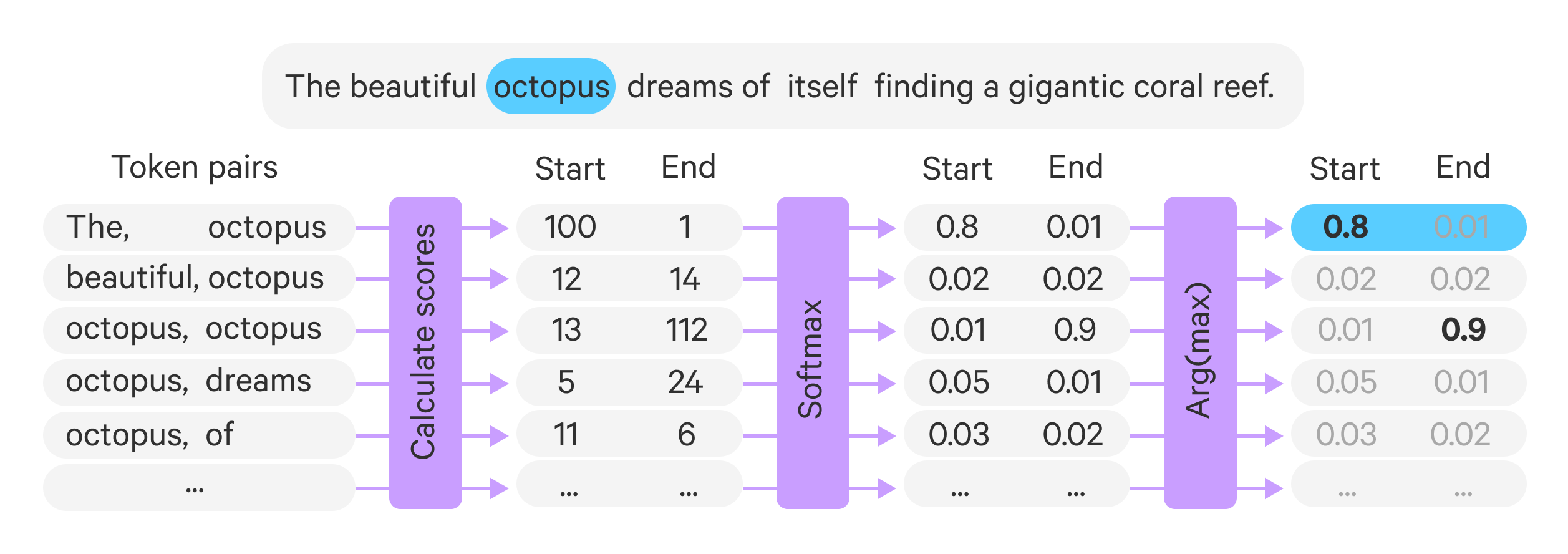
The SpanResolver is a lightweight convolutional network with two output channels. It takes as input the concatenation of the features of each token concatenated with the head token. Our example sentence yields the concatenations:
[[the; octopus], [beautiful; octopus], [octopus; octopus], [dreams, octopus], [of; octopus], [itself; octopus], [finding; octopus], [a; octopus], [gigantic; octopus], [coral; octopus], [reef; octopus]]Give the focus word “octopus” the SpanResolver will make two independent binary decisions for each pair indicating whether they are start or end of the span. Here the pair [the; octopus] should be classified as start and [octopus; octopus] as end, while the rest of the pairs are neither. The SpanResolver first concatenates each token with the target head token:
head = 3token_vecs = numpy.random.randint(0, 10, (5, 3))>>>array([[6, 7, 4],       [6, 5, 1],       [0, 5, 8],       [7, 9, 2],       [4, 5, 7]])
head_stack = numpy.tile(token_vecs[head], (token_vecs.shape[0], 1))head_stack>>>array([[7, 9, 2],       [7, 9, 2],       [7, 9, 2],       [7, 9, 2],       [7, 9, 2]])pairs = numpy.hstack((token_vecs, head_stack))>>>array([[6, 7, 4, 7, 9, 2],       [6, 5, 1, 7, 9, 2],       [0, 5, 8, 7, 9, 2],       [7, 9, 2, 7, 9, 2],       [4, 5, 7, 7, 9, 2]])
The SpanResolver then scores each pair as to how likely the pair is to be a start-head pair and an end-head pair, by running a stack of convolutional layers with two outputs for each position. Finally, we run the softmax function over the start and end scores to obtain the start and end probabilities for each token in the sentence. During prediction we make sure that the end token comes after the start, but during training we simply compute the cross-entropy and do not enforce any such order constraint.
Putting it together
Now that we understand the inner workings of the CoreferenceResolver and SpanResolver, let’s discuss how they fit together.
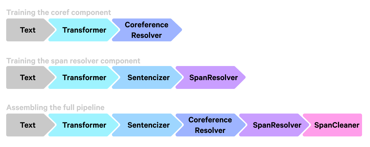
First, we create a training data set for the CoreferenceResolver turning the original span-level annotation into word-level by taking the head of each span. Then we train the CoreferenceResolver on the resulting data set to minimize the marginal log-likelihood of tokens that belong to the same cluster. For this phase the pipeline only includes a transformer to embed the documents and the coref component that contains the CoreferenceResolver.
Then we run the trained pipeline to annotate the training Doc objects with a number of SpanGroup objects prefixed with "coref_clusters" . For example we can access the first SpanGroup as doc.spans["coref_clusters_1"]. These SpanGroup objects are just groups of spans of length one i.e.: the head tokens. We often refer to these as “head clusters”.
We use the predicted head clusters as the training set for the SpanResolver. After the heads are generated we go through the OntoNotes training set and find for each head the shortest span that contains it. These head-span pairs then provide the training data for the SpanResolver that we train separately on the generated data. The SpanResolver is trained on the generated data with its own loss doing its own thing. This training stage trains a pipeline that additionally contains a sentencizer which is required for the SpanResolver.
After the second stage of training is done we use the spacy assemble command to put the CoreferenceResolver and the SpanResolver together into a final pipeline. When running the two components together the annotation doc.spans["coref_clusters_1"]now contains the full spans resolved from the heads.
Discussion and future plans
The term “coreference” actually encompasses a wide variety of linguistic phenomena. However, the system we have released is trained on the popular OntoNotes data set, which does not handle a couple of interesting cases.
One such example is the personal pronoun “you” as in ”You have to be ready for whatever you need to do, you know?”. Here the first two instances of “you” refer to some sort of generic person, whereas the third one is a discourse marker referring to an abstract listener.
Another example is with compound nouns where we refer to the compound modifier. So something like “Lemon grass got its name because it smells similar to our favorite citrus”. The “its” refers to the entire compound noun “Lemon grass”, but “our favorite citrus” refers back only to the modifier “Lemon”.
Both of these are examples of coreference phenomena not annotated in OntoNotes. For further reading on the debate around what coreference systems should cover we, recommend Can we Fix the Scope for Coreference? Problems and Solutions for Benchmarks beyond OntoNotes by Amir Zeldes.
For the time being the Natural Language Processing community does not have a consensus on what exactly a coreference resolution system should handle, and this is why the spaCy coreference pipeline is an end-to-end trainable pipeline that adapts to the provided training data sets as best as it can. However, machine learning based coreference systems — just like in other natural language processing or computer vision applications — can have a surprising performance degradation when taken out of their training domain. For interesting results concerning out-of-domain behavior of coreference resolution systems we recommend the paper OntoGUM: Evaluating Contextualized SOTA Coreference Resolution on 12 More Genres by Yilun Zhu, Sameer Pradhan and Amir Zeldes.
Finally, on the choice of architecture. The word-level approach we adopted is efficient and accurate, but is not appropriate for the use case where a reliable mention detector is available. When we have a component that can find spans of text that are probably mentions, we only need a span-level component to score these candidates. We are planning to implement a span-level option in the CoreferenceResolver following the bilinear scoring function based architecture that can take predicted mentions as input following Coreference Resolution without Span Representations by Yuval Kirstain, Ori Ram and Omer Levy. We are planning to use SpanFinder as mention-detector and chain it together with CoreferenceResolver .
Another limitation the CoreferenceResolver + SpanResolver pipeline has at the moment is the global and parallel nature of the processing. It scores all tokens against all other tokens at the same time using GPU parallelism. The implementation of such a strategy is really nice and straightforward, and is fast and accurate. The problem is the memory footprint. An alternative approach is to do greedy incremental clustering instead: scanning the document left-to-right and when a new mention is encountered either assigning it to an existing cluster, create a new cluster or ignore it. This approach can even be applied to sequential cross-document coreference resolution where documents are coming in as a stream.
Before you go!
Quite a long blogpost, right? Thank you for checking it out, and we hope that you’ve gotten a better understanding about how neural network based coreference systems work. If you are interested check out the experimental coreference resolution pipeline available in spacy-experimental v0.6.0. We have released the transformer-based English coreference pipeline trained on OntoNotes, which we currently call en_coreference_web_trf. For a more hands-on introduction how to use the pipeline, we will release a tutorial video soon! Finally, please let us know if you’ve encountered any bugs or you have suggestions for improvements! Hope we bump into each other on the web again!
Resources
- Experimental Coref Pipeline: The release contains a pre-trained spaCy pipeline that you can use right away!
- Experimental Coref Project: A project to train the components outlined in this post on OntoNotes, and basic usage instructions for the pipeline
- End to End Neural Coreference Resolution (Lee et al. 2017): The paper that laid the groundwork for our approach
- Word-level Coreference Resolution (Dobrovolskii 2021): The paper that directly informed our implementation


